Review of Proof-Writing - Start Doing Graph Theory

The purpose of this chapter

While I hope that these little sections at the beginning of each chapter are always useful, the note in this chapter is much more important to read!

It would be far too ambitious of me to hope to write a single chapter that will teach you how to write a proof. Entire books have been written on this subject. Here are a couple that have been made freely available online by their authors:

Book of Proof by Richard Hammack [48].

You can find it online at https://richardhammack.github.io/BookOfProof/.
An Infinite Descent into Pure Mathematics by Clive Newstead [77].

You can find it online at https://infinitedescent.xyz/.

A classic book that should also be mentioned is How to Solve It by George Pólya [84]. It is not a book about the method of writing a proof, but will give you advice on how to come up with an idea for it, which is maybe even more valuable.

Usually, when you learn proof-writing, you begin by proving statements that are mathematically easy, so you don’t have to struggle with two things at once. After you’ve done that, you might not yet be comfortable with writing proofs on topics that challenge you mathematically. If this is the level you’re at, then this chapter is for you.

I will try to prepare you for the kind of proofs you will encounter in this book by showing you how the general ideas of proof-writing specialize to graph theory. A proof is a proof in every area of math, but there are some ideas that show up in graph theory much more often than in number theory or real analysis, for example. When you get used to proofs in several areas of math, you will be an experienced mathematician. You’ll be able to jump into a new topic much more confidently.

So that you can benefit from this chapter early, I’ll limit myself to examples from the first part of this book (Chapter 1 through Chapter 4), but I will mention chapters later in the book where you’ll see more examples.

Conditional statements

In the moment when you first start trying to prove a theorem, you may not yet know how the proof will go. However, just from the statement of the theorem, you can have a rough overall idea of the strategy you need to take. This is a good way to fight “blank page syndrome”, where you’re staring at a problem and have no clue what to write!

So what do we look for in a statement? A big part of it is conditional statements: statements that can be expressed in the form “If $P$, then $Q$”. If you’re trying to prove such a statement, you can try:

A direct proof, where you assume that $P$ is true, and try to prove that $Q$ is true.
A proof by contrapositive, where you assume the negation of $Q$, and try to prove the negation of $P$. (This is a direct proof of the contrapositive, “If not $Q$, then not $P$”, which is an equivalent form of the original conditional statement.)
A proof by contradiction, where you simultaneously assume both $P$ and the negation of $Q$, and try to prove any statement you know is false.

A big reason why conditional statements are confusing to beginners is that the informal meaning of “if $P$, then $Q$” in the English language is under-specified. If you say a sentence like this in casual conversation, only context can determine what you mean in the case that $P$ is not true. Consider the following examples:

“If you’ve lived in Paris your whole life ($P$), you’re French ($Q$).” Here, $Q$ can still be true even if $P$ is false: many French people have never been to Paris.
“If you spend at least $50 ($P$), you will get free shipping ($Q$).” Here, the offer implies that you will not get free shipping unless you spend at least $50: when $P$ is false, $Q$ is also false.
“If you’re hungry ($P$), there’s pizza in the fridge ($Q$).” Here, the condition is irrelevant, and $Q$ is true regardless of the status of $P$.

In formal mathematics, an “if $P$, then $Q$” statement always goes hand-in-hand with an implicit “and if not $P$, then anything could be true”. It is an assertion that $Q$ is true, but limited only to situations where $P$ is true, without making any claim about situations where $P$ is false. When we want to talk about both situations, and say that when $P$ is false, $Q$ must also be false, the standard formulation is “$Q$ if and only if $P$”.¹

Even mathematicians are not perfect at maintaining this distinction in all circumstances. One place where you will often see the word “if” misused, from a formal point of view, is in definitions. Though I have avoided it in this book, it is common to see definitions phrased as, for example, “A walk $(x_0, x_1, \dots, x_l)$ is closed if $x_0 = x_l$.” All definitions should be read as if-and-only-if statements: a walk is closed if $x_0 = x_l$, and not otherwise.

Finally, let me say a bit about necessary conditions and sufficient conditions. This is another view of conditional statements. If the statement “If $P$, then $Q$” always holds, we say that $P$ is a sufficient condition for $Q$: knowing that $P$ is true is enough to know that $Q$ is true. We call $Q$ a necessary condition for $P$, in the sense that without $Q$ happening, $P$ can’t happen either: this is a paraphrase of the contrapositive, “If not $Q$, then not $P$”. We don’t always use these terms, though: we use them to emphasize specific ways of thinking about a conditional statement.

We say that $P$ is a sufficient condition for $Q$ to emphasize that we’re in a scenario where $Q$ is normally a difficult statement to evaluate, but $P$ is an easy-to-check test that can sometimes tell us that $Q$ is true. For example, Corollary 4.7 is a conditional statement where $P$ is “A graph $G$ with $n$ vertices has at least $n$ edges” and $Q$ is “$G$ contains a cycle”. Often, counting vertices and edges is much easier than investigating the graph’s structure to see if it has a cycle or not. If we count the vertices and edges and the hypothesis of Corollary 4.7 holds, then we can skip that investigation! The condition we’ve checked is sufficient to know that the graph has a cycle without looking for it.

We say that $Q$ is a necessary condition for $P$ in the reverse scenario: when $P$ is difficult to investigate, and $Q$ is a simple test. However, with necessary conditions, the test has a different meaning: we learn nothing if we check $Q$ and it is true, but if we check $Q$ and it is false, we learn that $P$ must also be false. For example, Proposition 2.2 tells us that if $G$ and $H$ are isomorphic, then $|V(G)| = |V(H)|$ and $|E(G)| = |E(H)|$. Determining whether two graphs are isomorphic is hard, but counting the vertices and edges is a simple initial test we can do. If $|V(G)| \ne |V(H)|$, or if $|E(G)| \ne |E(H)|$, we can skip the hard work: the necessary condition doesn’t hold, so $G$ and $H$ are definitely not isomorphic!

If we have an if-and-only-if relationship between $P$ and $Q$, then either statement is said to be a necessary and sufficient condition for the other. If we discover such a relationship, and one of the statements is a simple test, then we can consider the other statement to be easy to check as well. Knowing whether $P$ is true or false tells us all about $Q$, and vice versa.

Quantifiers

Whichever proof strategy you select, it will give you some goals to work toward, and some initial assumptions to work with. Usually, those goals and assumptions will contain quantifiers, which give you further structure. Quantifiers come in two types: existential and universal.

An existential quantifier is fancy terminology for a piece of a statement which says that some kind of object exists. The notation “$\exists x\in S, P(x)$” is shorthand for saying, “There exists an object $x$ in the set $S$ for which $P(x)$ is true.”

Typically, we prove such a claim by constructing an example; in simple cases, that just means writing down what it is. For example, suppose you want to prove the following statement: “The circulant graph $\operatorname{Ci}_8(3)$ is isomorphic to $C_8$.” Two graphs $G$ and $H$ are isomorphic if there exists an isomorphism between them: a function $\varphi \colon V(G) \to V(H)$ with certain properties. Your proof might begin by defining a function $\varphi$, and then checking that it has the properties that make it an isomorphism between $\operatorname{Ci}_8(3)$ and $C_8$.

I should also describe what happens when an existential statement is part of your assumptions. In that case, you get to summon up an object of the type being described, and start using it in your proof; this can be incredibly helpful! For example, suppose you are giving a direct proof of the following statement: “If a graph $G$ has an $x-y$ walk, then it has an $x-y$ path.” The existence of an $x-y$ walk is one of your assumptions: you get to assume that such a walk exists.

It’s often a good idea to describe the object in detail, giving names to its moving parts; you might begin by saying, “Let the sequence $(x_0, x_1, \dots, x_l)$ be an $x-y$ walk, with $x_0 = x$ and $x_l = y$.” Later on in the proof, you will get to manipulate the vertices $x_0, x_1, \dots, x_l$, and use facts about them that are based on the definition of an $x-y$ walk.

Moving on, a universal quantifier says that a statement is always true: it is a universal rule. The notation “$\forall x \in S, P(x)$” is shorthand for saying, “For all objects $x$ in the set $S$, the statement $P(x)$ is true.”

What if the set $S$ is the empty set?

In that case, a statement about all elements of $S$ is automatically true, because there’s nothing to check: we say it is vacuously true.

We don’t generally make such statements on purpose, but we might get them as a special case of a more general theorem.

To prove such a statement, we need an argument that applies to every element of $S$ at once. There is a standard way to phrase such an argument: it is to choose an arbitrary element $x \in S$, assuming nothing else about it. Then, your goal is to prove that $P(x)$ is true. This can be easy or hard, but look on the bright side: in this scenario, you both get to start with an element $x\in S$ to work with, and get an idea of how you want your proof to end!

For example, suppose you want to prove the following statement: “For all integers $n\ge 3$, the cycle graph $C_n$ is connected.” You would begin by taking an integer $n\ge 3$, and writing the rest of your proof for that value of $n$. As long as you don’t accidentally sneak in any further assumptions about $n$, your argument will apply to every integer you could have chosen.

The case I find most frustrating is the case of assuming a “for all” statement, because you can’t do anything with it when you begin. For example, suppose you have a graph $G$ for which you’ve made the assumption, “All cycles in $G$ have an even length.” (See Chapter 13 to learn more about such graphs.) You can’t do anything right away—it’s only once you encounter a cycle in $G$ that this assumption “triggers” and tells you that the length of the cycle is even. It’s possible that $G$ has no cycles, in which case you will never get to use the assumption.

To give you an overview of the situation at a glance, Figure A.1 describes what happens to both types of quantifiers in both cases: when you assume them, and when you prove them. Since some cases are easier to deal with than others, you can try to change which case you have to deal with by changing your approach.

You could try a different proof method that changes what you have to do: for example, instead of proving a statement, you might assume its negation.
You could use a theorem which gives an alternate characterization of an object, with a different type of quantifier.

In more complicated statements, you will have to juggle both kinds of quantifiers at once. An especially important combination to look at is the combination $\forall x, \exists y$: “For every $x$, there exists a $y$.” This is a very demanding statement to prove, because you must present an example of $y$, which might have to depend on $x$; however, you can’t make any assumptions about $x$. Let me give you some examples to compare:

“The circulant graph $\operatorname{Ci}_8(3)$ is isomorphic to $C_8$” is a concrete, purely existential statement: no universal quantifiers at all. You can prove that an isomorphism exists by writing down what it is and checking the conditions.
“For all odd $n\ge 3$, the circulant graph $\operatorname{Ci}_n(2)$ is isomorphic to $C_n$” has a universal quantifier on $n$, but an existential quantifier hidden inside the word “isomorphic”. You might still be able to write down an isomorphism, but you will have to write it down as a formula in terms of $n$.
“Every connected $n$-vertex graph $G$ in which all vertices have degree $2$ is isomorphic to $C_n$” is even trickier: it has a universal quantifier on a graph $G$, which is a much more complicated object than a number!

You will not be able to write down an isomorphism, not even with the aid of formulas, because you can’t plug a graph $G$ into a formula. In your proof, you might describe a general strategy for finding an isomorphism, and check that it always works.

This situation is part of the reason why algorithms play a big role in graph theory: a common way to prove that something exists is to give an algorithm for finding it. Theorem 8.3 and Theorem 8.4 are good examples of this technique early in the book.

I should also warn you that often, universal quantifiers are omitted in the statement of a theorem. If the statement of a theorem contains variables that don’t have a quantifier attached, this usually means that the theorem should be true for all possible values of those variables; the scope should hopefully be clear from context.

I try to avoid doing this too much, but consider for example Corollary 4.7, which I guess I shouldn’t go back and edit because then I won’t be able to use it as an example here. The full statement of the corollary is: “If $G$ has $n$ vertices and at least $n$ edges, then $G$ contains a cycle.” Neither $G$ nor $n$ is quantified, so we interpret both of them as having hidden universal quantifiers on them. The statement should be true for all graphs $G$ and for all integers $n\ge 1$.

How do we know what kind of variables $G$ and $n$ are?

Part of this is convention: $G$ usually refers to a graph and $n$ usually refers to an integer. Part of this is context: $G$ is mentioned as having vertices and edges, so it should be a graph, and $n$ is the number of vertices in $G$, so it can only be a positive integer.

Unpacking definitions

Quantifiers, implications, and many other parts of a statement can be tucked away inside a definition where you can’t easily see them. For example, it is not obvious from reading “$G$ and $H$ are isomorphic” that it’s existential ($\exists$) statement: that there exists a function $\varphi \colon V(G) \to V(H)$ which is an isomorphism. (Inside the definition of an isomorphism, more quantifiers are tucked away!)

What are the quantifiers in “$G$ is connected?”

It’s a $\forall\exists$ statement: for every two vertices $x,y \in V(G)$, there exists an $x-y$ walk.

What are the quantifiers in “The maximum degree of $G$ is $k$?”

It has two parts: a $\forall$ statement that every vertex has degree at most $k$, and an $\exists$ statement that there exists a vertex of degree $k$. (More on such statements later!)

This means that there’s an important first step you have to keep in mind whenever you write a proof: you must unpack all the definitions you’re working with to get at the moving parts inside them!

Let’s look at an example of this: the proof of Lemma 3.3. This lemma claims that the relation $\leftrightsquigarrow$ on the vertices of a graph $G$ is an equivalence relation, where $x \leftrightsquigarrow y$ is defined to mean that there is an $x-y$ walk in $G$.

To begin with, we are proving that something is an equivalence relation. By definition, an equivalence relation is a relation which is reflexive, symmetric, and transitive. So right away, we know that our proof will have three parts, one where we prove each part of the definition.

Let’s look at just one of these: proving that $\leftrightsquigarrow$ is symmetric. The definition of this is that for all $x$ and $y$ (which, in this case, are vertices of $G$), if $x\leftrightsquigarrow y$, then $y\leftrightsquigarrow x$.

Assuming that we choose to write a direct proof (which there’s no reason not to do), which quadrant of Figure A.1 are we in?

The top right quadrant: we are proving a universal statement about all pairs of vertices $x,y \in V(G)$.

Therefore we begin by choosing arbitrary vertices $x,y \in V(G)$. We assume that $x\leftrightsquigarrow y$ is true, and set ourselves a goal: to prove that $y\leftrightsquigarrow x$ is true. At this point, we must also unpack the definition of $x\leftrightsquigarrow y$. We are assuming that there is an $x-y$ walk in $G$; we are proving that there is a $y-x$ walk in $G$.

Which quadrants of Figure A.1 do these fall under?

The bottom two quadrants: both the assumption we make about $x$ and $y$ and the property we want to prove are existential statements. We get to summon an $x-y$ walk out of nowhere, but we will have to construct a $y-x$ walk.

It is not very helpful to use the existence assumption merely by saying something like, “Let $W$ be an $x-y$ walk in $G$.” To get anything useful out of the assumption, we should unpack the definition of an $x-y$ walk. We say, “Let the sequence $(x_0, x_1, \dots, x_l)$ be an $x-y$ walk, with $x_0 = x$ and $x_l = y$.”

Looking ahead, we see that we’ll want to define a new sequence of vertices, which we will then prove is a $y-x$ walk. It is only at this point that we get to the problem-solving step of the proof! To figure out how to get a $y-x$ walk out of an $x-y$ walk, we might look at some small examples to get a feeling for the problem. With experience comes an “intuition” for things to try, which is just a way to say that you’ve seen similar problems before and have some guesses about what might work.

To summarize, here is the “scaffolding” of a proof that $\leftrightsquigarrow$ is symmetric; only the sections with “…” are left for us to figure out. (Not every proof is as heavy in definitions, and so you won’t always have as much unpacking to do.)

Proof. Let $x$ and $y$ be two arbitrary vertices, and suppose that $x \leftrightsquigarrow y$: that there is a $x-y$ walk in $G$. Our goal is to prove that there is also a $y-x$ walk in $G$.

Let $(x_0, x_1, \dots, x_l)$ be an $x-y$ walk (with $x_0 = x$ and $x_l = y$). Then define a new sequence of vertices by …

This sequence of vertices starts at $y$, ends at $x$, and consecutive vertices in the sequence are adjacent because …, proving that it is a $y-x$ walk.

Since a $y-x$ walk exists, we conclude that $y \leftrightsquigarrow x$. Since this is true for all pairs of vertices $x,y \in V(G)$, we conclude that that $\leftrightsquigarrow$ is symmetric. ◻

I should also mention that there is a danger to unpacking too far. If you unpack every definition you can, you are forced to write a “low-level” proof that works with the fundamental notions of graph theory. The alternative is a “high-level” proof, where you stop early to apply a theorem you know to an object without unpacking it.

For example, in Chapter 4, we gave Theorem 4.4 a low-level proof: we proved that a cycle exists by listing out the vertices of a walk representing it. Later, we gave Corollary 4.7 a more high-level proof: we proved that a cycle exists by applying Theorem 4.4, without interacting directly with the definition of a cycle.

Optimization problems

Many definitions in graph theory involve solving an optimization problem: they are phrased in terms of the biggest or smallest thing of a certain type. In the first part of the textbook, this includes:

The distance between two vertices $x$ and $y$: the length of the shortest $x-y$ walk.
The minimum and maximum degree of a graph $G$: the smallest and largest, respectively, of the degrees of the vertices of $G$.

When we say, “The distance between vertices $x$ and $y$ is $5$,” we are making two separate claims. First, we are saying that there is in fact an $x-y$ walk of length $5$. Second, we are saying that this is the shortest walk: all $x-y$ walks have length at least $5$. The first claim is an existential ($\exists$) statement, and the second claim is a universal ($\forall$) statement.

What statement about the distance $d(x,y)$ do we make if we only say that there is an $x-y$ walk of length $5$?

This is equivalent to saying that $d(x,y) \le 5$. The distance can’t be longer than $5$, because we’ve already found walk of length $5$, but it might be shorter.

What statement about the distance $d(x,y)$ do we make if we only say that that all $x-y$ walks have length at least $5$?

This is equivalent to saying that $d(x,y) \ge 5$. We can’t do better than $5$, but we don’t know if we can actually achieve $5$.

What we see for proofs about the distance between two vertices is true in general. An upper bound on a minimization problem is an existential statement: we can prove it by giving a single example of a solution that achieves that bound. A lower bound on a minimization problem is a universal statement: we can prove it by proving that no solution can do better. For maximization problems, the situation is reversed.

Let’s look at an example.

Proposition A.1. Let $G$ be the graph with vertex set $V(G) = \{1,2,\dots,100\}$ in which two vertices $x$ and $y$ are adjacent if and only if $|x-y|$ is the square of a positive integer. (For example, vertices $7$ and $71$ are adjacent, because $|7 - 71| = 64 = 8^2$.)

Then $G$ has maximum degree $\Delta(G)=14$.

Proof. First, we prove that a vertex of degree $14$ exists, by example. The vertex $50$ is adjacent to the $14$ vertices \[1, 14, 25, 34, 41, 46, 49, 51, 54, 59, 66, 75, 86, 99.\] We don’t have to check them all by hand: these are the vertices $50-k^2$ for $k=1,2,\dots,7$ and $50+k^2$ for $k=1,2,\dots,7$. All we have to do is to check that the extreme values $50 - 7^2 = 1$ and $50 + 7^2 = 99$ still fall within $V(G)$.

This example proves that $\Delta(G) \ge 14$; to prove that $\Delta(G) \le 14$, we prove that all vertices have degree at most $14$.

Let $x$ be an arbitrary vertex. From the example we looked at, we can see that to find the degree of $x$, we need to count how many values of the form $x - k^2$ or $x + k^2$ fall with in the range $\{1,2,\dots,100\}$. Let $a$ be the largest integer such that $x - a^2 \ge 1$, and let $b$ be the largest integer such that $x + b^2 \le 100$; then the neighbors of $x$ are $x - 1^2, x - 2^2, \dots, x - a^2$ and $x + 1^2, x + 2^2, \dots, x + b^2$, and $x$ has degree $a+b$.

What is the largest possible value of $a$?

It is $9$: even if $x$ is as large as possible, that is if $x=100$, then $x - 10^2$ is still not in the range $\{1,2,\dots,100\}$.

Similarly, we can prove that the largest possible value of $b$ is $9$, giving us an upper bound of $9+9=18$ on the degree of $x$, and on the maximum degree. But that’s not good enough; we wanted $\Delta(G) \le 14$, not $\Delta(G) \le 18$.

What prevents us from making both $a$ and $b$ this large simultaneously?

To get $a$ to reach $9$, we need $x$ to be close to the end of the range. To get $b$ to reach $9$, we need $x$ to be close to the start of the range.

We know that having $a=7$ and $b=7$ are possible when $x=50$, so let’s rule out the remaining possibilities. If $a \in \{8,9\}$, then $x - 8^2 \ge 1$, so $x$ is at least $1 + 8^2 = 65$; but now, since $65 + 6^2 = 101$ is too big, we learn that $b \le 5$. Similarly, if $b \in \{8,9\}$, then $x + 8^2 \le 100$, so $x$ is at most $100 - 8^2 = 36$; but now, since $36 - 6^2 = 0$ is too small, we learn that $a \le 5$. So in these cases, no better solution than $a+b = 9+5 = 14$ or $a+b=5+9=14$ is possible.

Is $(a,b) = (9,5)$ or $(a,b)=(5,9)$ actually achievable?

No: for example, $a=9$ requires $x \ge 82$, and $b=5$ requires $x \le 75$. This is fine for our proof: we are done with the stage that proves existence, now we are only ruling out options, and we don’t care about ruling out options that don’t contradict the upper bound $\Delta(G) \le 14$ we want.

When $a \in \{8,9\}$ or $b \in \{8,9\}$, we have $\deg(x) = a + b \le 14$. But if $a \le 7$ and $b \le 7$, we also have $\deg(x) = a + b \le 14$. Therefore $\deg(x) \le 14$ no matter what $x$ is. This tells us that $\Delta(G) \le 14$, which completes the overall proof. ◻

In Chapter 5, the diameter of a graph $G$ is introduced: the largest distance between two vertices of $G$. The definition of diameter has one optimization problem nested inside another! This means that both lower and upper bounds on the diameter of a graph unpack to statements with multiple quantifiers.

For example, suppose we want to prove that the diameter of $G$ is at most $k$. Then we want to prove that $d(x,y) \le k$ for all pairs of vertices $x,y$, which is a $\forall\, \exists$-type statement: for all $x$ and $y$, there exists an $x-y$ walk of length at most $k$.

What if we try to prove that the diameter of $G$ is at least $5$?

This will be an $\exists\,\forall$-type statement: we want to prove that there exist vertices $x$ and $y$ such that all $x-y$ walks have length at least $5$.

Here are some of the notable optimization problems introduced later in the book:

The maximum matching problem and the minimum vertex cover problem, introduced in Chapter 13.
The independence number $\alpha(G)$ and clique number $\omega(G)$, defined in Chapter 18.
The vertex and edge coloring problems studied in Chapter 19 and Chapter 20.
The connectivity $\kappa(G)$ and several related parameters, defined in Chapter 26.

Algorithms

Algorithms play a role in graph theory for two reasons.

First of all, there are many applications of graph theory in software, so computer scientists think about graph algorithms.

Second, even pure mathematicians that don’t care about computer science at all can be interested in graph algorithms as an aid in proof-writing. One way to prove that an object exists is to give an algorithm for finding it.

In both cases, but especially in the second case, it’s important for the algorithm to be accompanied by a proof of correctness. In most respects, this is a proof like any other. There are a few proof techniques that are unusually common when dealing with algorithms, which we’ll see in a moment. Before that, there’s one feature of the proof that I want to point out, because it’s easy to miss if you’ve never thought about it before. It is important to prove that the algorithm eventually stops, and doesn’t just keep iterating forever!

In the first part of the book, there is only one notable algorithm: breadth-first search, which we use to compute distances in a graph at the end of Chapter 3. Breadth-first search continues to be useful in algorithms throughout this book: as late as Chapter 28, we return to it to find a shortest path in a residual network. In this algorithm, the stopping condition is relatively straightforward. In each step, we either explore at least one new vertex, or we stop because we didn’t find any new vertices. We cannot keep exploring new vertices forever: eventually, we run out of vertices in the graph to explore!

Such situations are common, but not universal. In this textbook, the most sophisticated proof that an algorithm stops is Theorem 28.7, for an algorithm to find maximum flows. In that case, the algorithm deals with real numbers, and it’s possible to keep increasing a real number forever even if there’s an upper bound on the number; this is what makes the analysis tricky!

To see a tricky proof that an algorithm stops that only needs topics from the first part of the book, let me give an example from the 2019 Princeton University Mathematics Competition (PUMaC): problem 1 from the individual final round in Division A [86]. The problem does not talk about algorithms, but it describes an iterated procedure performed on a graph, so many of the same ideas come up. Here it is:

Problem A.1. Given a connected² graph $G$ and cycle $C$ in it, we can perform the following operation: add another vertex $v$ to the graph, connect it to all vertices in $C$ and erase all the edges from $C$. Prove that we cannot perform the operation indefinitely on a given graph.

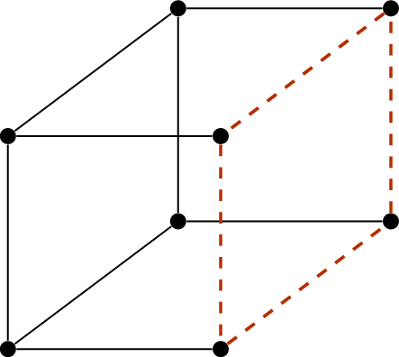
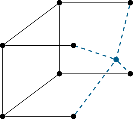
An example of this operation is shown in Figure A.2. Since the graph gets bigger and bigger every time we perform the operation, it’s not at all obvious that we’ll eventually have to stop!

To solve the problem, we’ll need two lemmas.

Lemma A.2. After the operation in Problem A.1 is performed on a connected graph, the result is another connected graph.

Proof. Let $G$ be the graph we started with and let $H$ be the result of performing the operation.

For any two vertices $x,y \in V(G)$, there is an $x-y$ walk in $G$, because $G$ is connected. We can turn this $x-y$ walk in $G$ into an $x-y$ walk in $H$, even though not all edges of $G$ are still present in $H$. Every time that the walk goes from a vertex $u$ to a vertex $w$ along an edge of $C$, replace that step by two steps, $u$ to $v$ to $w$.

This proves that all vertices of $V(G)$ are in the same connected component of $H$. In $H$, there is one more vertex: the vertex $v$ we added. It is in the same component as the other vertices, because it is adjacent to the vertices on $C$; this proves that $H$ is connected. ◻

Lemma A.2 is a good example of proving an invariant of an algorithm (not to be confused with a graph invariant). By showing that some property (in this case, the connectedness of the graph) does not change after we perform the operation once, we can conclude that it never changes. In this case, it follows from Lemma A.2 that no matter how many times we perform the operation in Problem A.1, we will have a connected graph.

We can obtain another invariant by counting the vertices and edges.

In Figure A.2, what is the number of vertices before and after the operation, and what is the number of edges?

The number of vertices goes from $8$ to $9$. The number of edges remains at $12$: we deleted $4$ edges on the cycle, but added $4$ edges from the vertices of the cycle to the new vertex.

This example is probably enough to guess what happens in general:

Lemma A.3. After the operation in Problem A.1 is performed on a graph with $n$ vertices and $m$ edges, the result is a graph with $n+1$ vertices and $m$ edges.

Proof. The new graph has $n+1$ vertices because $1$ vertex is added and none are removed.

Let the cycle $C$ used in the operation have length $k$; then $C$ has $k$ vertices and $k$ edges. Deleting the edges of $C$ reduces the number of edges from $m$ to $m-k$, but adding an edge from $v$ to each vertex of $C$ increases the number of edges from $m-k$ back to $m$. ◻

Technically, the number of vertices is not an invariant of the algorithm, but a monovariant: rather than always staying the same, it increases in a predictable way.

Armed with these two lemmas, we can explain why the operation can’t be continued forever.

Suppose that we could perform the operation $100$ times on the cube graph. What can you say about the result?

The result must be a connected graph (by Lemma A.2) with $108$ vertices and $12$ edges (by Lemma A.3).

Why is this ridiculous?

In a graph with $108$ vertices and $12$ edges, there are not even enough edges to give every vertex a neighbor! The graph must have many different connected components which are isolated vertices; it certainly cannot be connected.

Generalizing this logic, suppose that we start with a connected graph $G$ that has $n$ vertices and $m$ edges. Assume for the sake of contradiction that we can perform the operation at least $2m$ times. When this is done, we have a connected graph $G$ (by Lemma A.2) with $2m+n$ vertices and $m$ edges (by Lemma A.3).

To see the problem clearly, apply the handshake lemma (Lemma 4.1). If every vertex in $G$ has degree at least $1$, then the sum of all $2m+n$ degrees is at least $2m+n$, but the handshake lemma says that the sum of degrees is only $2m$. Therefore $G$ must have some vertices of degree $0$. Each such vertex is a connected component all by itself: somehow, $G$ is not connected! This is a contradiction, so it must be impossible to perform the operation $2m$ times.

In fact, using techniques from Chapter 10, we can determine the exact number of times we can perform the operation before we have to stop. When we are forced to stop, we must have a graph that is connected but has no cycles: by Theorem 10.2, this graph must be a tree! A tree with $m$ edges has $m+1$ vertices, so if we started with a connected graph that has $m$ edges and $n$ vertices, we will be able to perform the operation $m-n+1$ times: no more, and no less.

The extremal principle

Not all proofs of existence are algorithms that tell you how to construct the object we want. There are many proof techniques that let us prove something exists without giving us any clues about how to find one. (For example, in Theorem 18.5, we prove that a graph with a certain property exists by showing that a randomly chosen graph has a positive probability of having that property.)

A notable proof technique of this type is the extremal principle. In the first part of the book, there are two examples of its use:

In Theorem 3.1, to prove that an $x-y$ path exists, we chose a shortest $x-y$ walk, and then proved that it represents a path.
In Theorem 4.4, to prove that a cycle exists, we chose a longest path, and then proved that an initial segment of that path can be turned into a cycle.

In general, the extremal principle is a way we can make use of an assumption that something exists (as in the bottom left quadrant of Figure A.1) and strengthen that assumption for free. Instead of taking an arbitrary object of that type, we take an object which is as good as possible by some measure.

There are two caveats to this. First of all, you have to know that there are objects of that type. When we chose a shortest $x-y$ walk in the proof of Theorem 3.1, for example, the existence of $x-y$ walks was one of our assumptions. If it was not, then the proof would not be valid: we can’t take a shortest $x-y$ walk if there’s a possibility that $x$ and $y$ are not in the same connected component.

When we chose a longest path in the proof of Theorem 4.4, how did we know that a path exists?

If nothing else, a graph with at least one vertex should have a path of length $0$. (With the assumption that the graph has minimum degree $2$, we can even guarantee slightly longer paths than this!)

Second, it must be guaranteed that there is a best object, however you decide to judge “best”. Ties are okay, but when there are infinitely many options to choose from, it’s possible that no matter which object you choose, there’s a better one. In graph theory, we are usually dealing with non-negative integers. In that case, it’s always okay to pick the smallest value (as in the case of a shortest $x-y$ walk). In situations where there’s an upper bound on the value, we can also pick the largest; however, that’s not valid in general.

Why is there guaranteed to be a longest path in any graph?

In a graph with $n$ vertices, a path can also contain at most $n$ vertices, which means that it can have length at most $n-1$. (There’s not necessarily a path of length $n-1$; this is just an upper bound.)

When should you consider using the extremal principle? Although you could try using it at any time, I’ve found that there’s a specific kind of situation where it’s convenient to use: when you can imagine doing something over and over again, the extremal principle can let you “skip to the end” of that process. That’s vague, so let me explain how it works in the two examples of this section.

To prove Theorem 3.1, you can imagine taking an $x-y$ walk and cleaning it up to make it represent an $x-y$ path, step by step. How can we do that? Well, an “un-path-like” thing for a walk to do is to revisit a vertex $z$. Whenever the walk does that, we can eliminate a visit to $z$ by skipping the segment of the walk between the first visit to $z$ and the last. Every time we do this, it makes the walk shorter. Therefore if we skip ahead to an $x-y$ walk that is as short as possible, it must not be possible to do this again.

To prove Theorem 4.4, you can imagine walking around the graph arbitrarily (but without backtracking along the same edge) until you come back to a vertex. When you’ve visited a vertex for a second time, the trajectory from your first to your second visit must form a cycle. How can we skip ahead to the end here? Well, every time we don’t come back to a vertex, we end up making a longer and longer path. So if we skip ahead to the longest path in the graph, we’ll be forced to come back to a vertex in the very next step.

Practice problems

Rewrite each of the following statements to make the quantifiers and logical implications inside it explicit.
1. Two isomorphic graphs always have the same number of edges.
2. Every $n$-vertex graph in which all vertices have degree at least $\frac{n-1}{2}$ is connected.
3. Every graph with more edges than vertices has a vertex of degree at least $3$.
4. The difference between minimum and maximum degree in a graph can be arbitrarily large.
Find the logical negation of each of the following statements, simplifying as much as possible so that no negations of complicated clauses are left. (It is okay if you are left with elementary negations like “$x$ is not adjacent to $y$”.)
1. Every $k$-vertex subgraph of $G$ has at most $k$ edges.
2. There is a set of $k$ vertices in $G$ with no edges between them.
3. There is a vertex in $G$ adjacent to all other vertices.
4. For all $n\ge 1$, if an $n$-vertex graph contains no copies of $G$, then it can have at most $\frac13 n^2$ edges.
5. For every vertex $x$ of $G$, there is another vertex $y$ such that every $x-y$ walk in $G$ has length at least $10$.
6. $G$ contains two vertices $x$ and $y$ such that for every vertex $z$ other than $x$ or $y$, if $z$ is adjacent to $x$, then $z$ is also adjacent to $y$.
7. Every graph theorist has a friend that knows somebody the graph theorist doesn’t know.
8. Every textbook has a practice problem that cannot be solved.
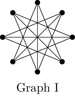
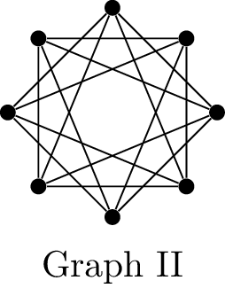
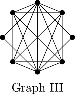
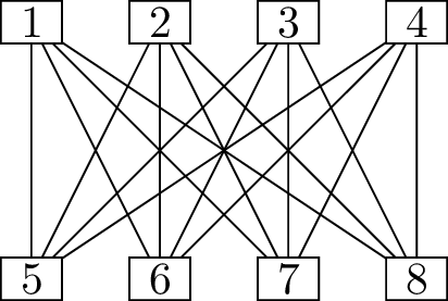
Use the three graphs below to answer the questions that follow.
1. If $G$ is a planar graph with $n \ge 3$ vertices, we know that $G$ has at most $3n-6$ edges. Using this condition and no other properties of planar graphs, what can we say about graphs I, II, and III?
2. If $G$ is a graph with $n \ge 3$ vertices and minimum degree at least $n/2$, we know that $G$ is Hamiltonian. Using this condition and no other properties of Hamiltonian graphs, what can we say about graphs I, II, and III?
3. A connected graph $G$ is Eulerian if and only if every vertex has an even degree. Using this condition and no other properties of Eulerian graphs, what can we say about graphs I, II, and III?
1. Prove that the circulant graph $\operatorname{Ci}_8(3)$ is isomorphic to the cycle graph $C_8$.
2. Prove that for all odd $n\ge 3$, the circulant graph $\operatorname{Ci}_n(2)$ is isomorphic to $C_n$.
3. Prove that for even $n \ge 4$, the circulant graph $\operatorname{Ci}_n(2)$ is not isomorphic to $C_n$.
Find the error in this proof of the statement “Graphs never have edges”.

Let $G$ be any graph, and let $x$ be an arbitrary vertex. Let $(x, x_1, x_2, \dots, x_l)$ be the longest walk beginning at $x$.

If there is an edge $xy$ incident to $x$, then the walk $(x, y, x, x_1, x_2, \dots, x_l)$ is a longer walk beginning at $x$. That’s a contradiction, because we assumed that we took the longest such walk. So the assumption that the edge $xy$ exists is incorrect: there are no edges incident to $x$. In other words, $x$ has degree $0$.

Since $x$ was an arbitrary vertex, all vertices of $x$ have degree $0$: in other words, the graph $G$ has no edges at all!
Write down a scaffolding for a direct proof of the claim “If a graph $G$ is isomorphic to its complement $\overline G$, then it is connected.”

That is, unpack all the definitions in the claim and identify all the quantifiers and logical implications. Then, write down all the assumptions and initial definitions you should make, as well as the conclusions you should eventually draw. You don’t have to fill in the details of how to get from the start to the end.
Prove that the graph shown below has diameter $2$:
Starting from the complete graph $K_{10}$, you repeatedly perform the following operation: select $4$ vertices of the graph, and toggle the presence of all $6$ edges between them (removing them if they are absent, and adding them if they are present).

Can you ever end up removing all edges of the graph?
A $P_3$-free graph is a graph that does not have the path graph $P_3$ as an induced subgraph. In other words, if you pick $3$ vertices inside a $P_3$-free graph, there will never be exactly $2$ edges between them: there could be $0$ edges, a single edge, or all $3$ edges.
1. Let $G$ be a $P_3$-free graph, and let $\sim$ be the adjacency relation in $G$: $x \sim y$ if and only if $xy \in E(G)$.
  
  Prove that $\sim$ is an equivalence relation on $V(G)$.
2. What does this tell us about the structure of $G$? Describe what a connected component of $G$ can look like.

Footnotes

Thus, a mathematician would write, “You will get free shipping if and only if you spend at least $50.”↩︎
The problem statement on the PUMaC website does not say that $G$ is connected, but the official solution assumes a connected graph. If $G$ is not connected, the same argument can be applied to each connected component. I’ve decided to add the assumption just so that we can skip this step.↩︎