In this chapter, we will not yet see any of the big theorems about
matchings. Here, we will only lay the foundations and begin to study
bipartite graphs, matchings, and vertex covers.
I have gone to some trouble in this textbook to postpone the
definition of bipartite graphs until this chapter. This is done for two
reasons. First, I do not want the first few chapters to be overloaded
with definitions and nothing but definitions—as much as I can help it,
at least. Second, I do not want to give a definition when we have no use
for it. This is because, to the extent I can, I want the definitions we
make and the questions we ask about them to seem like reasonable
definitions we make and reasonable questions to ask.
As a result, it is only now that I define bipartite graphs, because
now we can ask the bipartite matching problem. Here, it is reasonable to
ask whether (and in which way) a graph is bipartite, and so I hope that
the definitions and initial theorems do not feel pointless.
Two chess puzzles
The title of this section may be a slight exaggeration; you will not
need to know the rules of chess. These are, instead, two puzzles about
placing pieces on a chessboard.
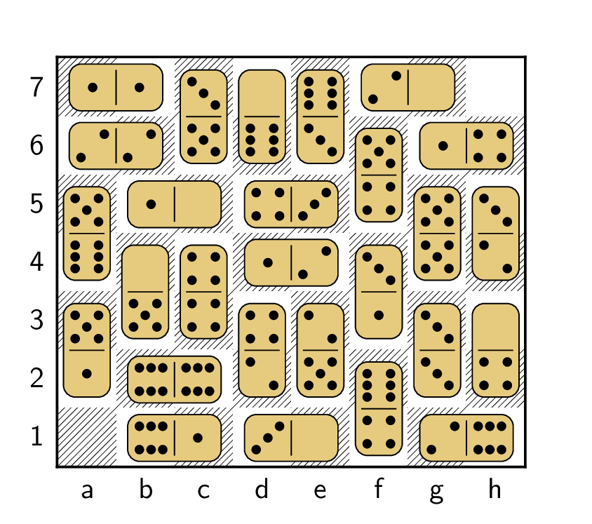
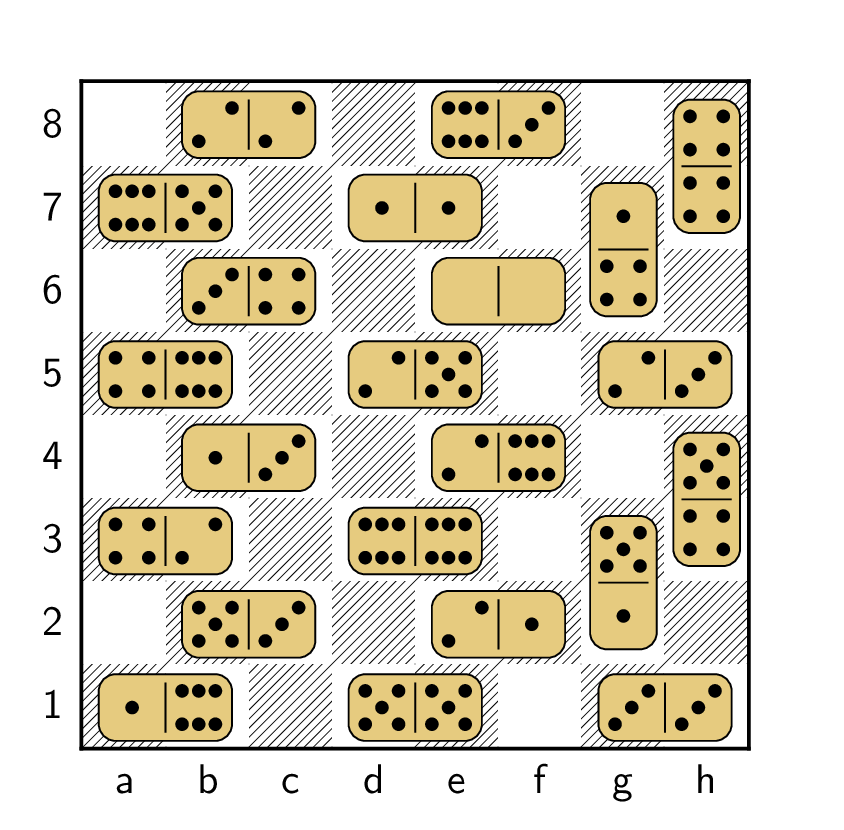
The first is a classic puzzle about placing dominoes on a chessboard.
A complete set of dominoes has \(28\)
dominoes; enough to completely cover an \(8\times 7\) grid. If I take away one
domino, then it’s possible to cover every square of the grid except for
two opposite corners: Figure 13.1(a)
shows one of many solutions.
But the standard chessboard is \(8\times
8\). So suppose you have \(31\)
dominoes: a complete set with three extras. Can you cover every square
of the \(8\times 8\) chessboard except
for two opposite corners?
Dominoes on a \(8\times 7\)
chessboardRooks on a chessboard
Placing pieces on a chessboard
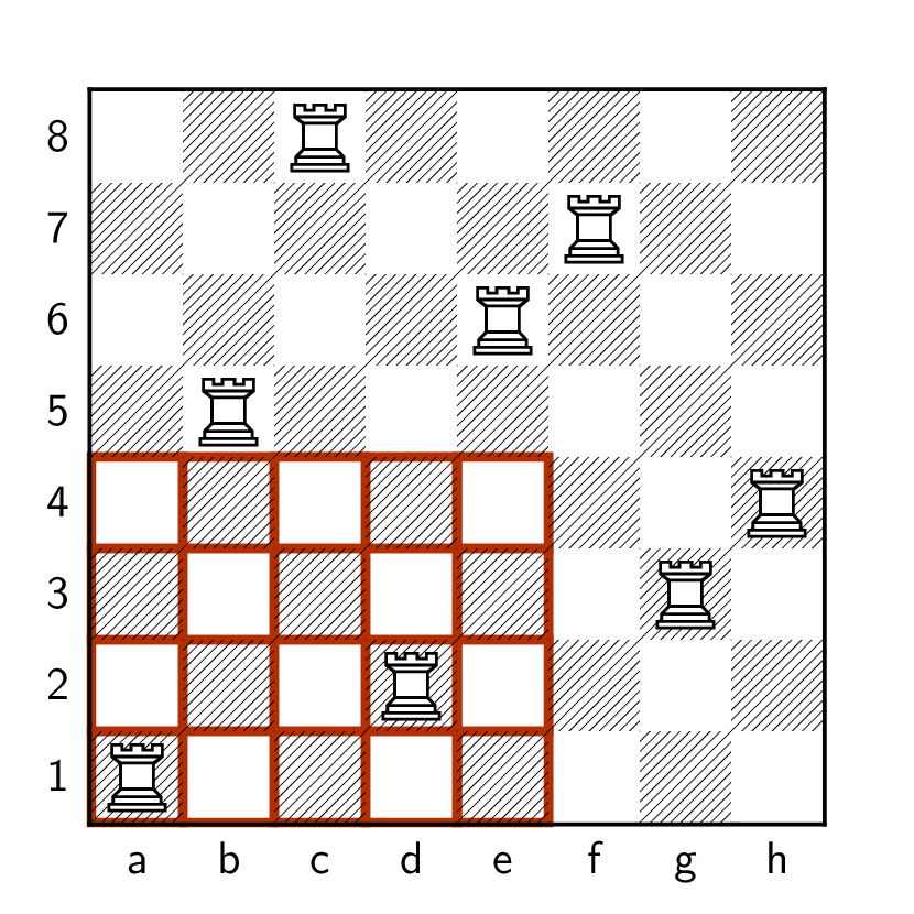
A second puzzle is shown in Figure 13.1(b). Here, we
place \(8\) rooks on a chessboard. A
rook can move any number of spaces horizontally or vertically; we don’t
want the rooks to get in the way of each other, so we want to place them
so that no two rooks are in the same row or column.1
I’ll add a condition to make this more difficult in a moment, but
first…
How many ways are there to place \(8\) rooks on an \(8\times 8\) chessboard so that no two rooks
are in the same row or column?
There are \(8! =
40\,320\) ways.
If we pick a column for the rook in row 1, then the rook in row 2,
and so on, then we will have \(8\)
options for the first rook, \(7\) for
the second rook, \(6\) for the third
rook, and so forth. By the product principle, we can multiply these
numbers together, getting \(8\cdot 7\cdot6
\cdot5\cdot4\cdot3\cdot2\cdot1\) or \(8!\) arrangements.
Now I can ask you the real puzzle. Suppose we exclude the \(4 \times 5\) area highlighted in Figure 13.1(b). Is it still possible to place
\(8\) rooks on the chessboard, still in
different rows and columns, so that this area remains empty?
We will be able to answer both questions with the tools in this
chapter. But first, let’s take a moment to ask the question we’ve been
asking since Chapter 1: how do we model each
puzzle with a graph? In both cases, there are actually two reasonable
approaches!
Let’s start with the domino puzzle. We’ve already seen a tiling
puzzle in Chapter 1, and we can model this
puzzle in the same way. Create a graph with a vertex for each valid way
to place a single domino: on an \(8\times
8\) chessboard with two opposite vertices removed, there will be
\(108\) vertices. Then, add an edge
between two vertices if they represent incompatible placements: dominoes
that share a square of the board. To place \(31\) dominoes, we are looking for a \(31\)-vertex independent set: a set
of \(31\) vertices that do not have any
edges between them.
As we will see in Chapter 18,
finding independent sets is a hard problem. So let’s instead take a
different graph to start with: the \(8\times
8\) grid graph \(G(8,8)\), with
vertices \((1,1)\) and \((8,8)\) removed.
If we model the chessboard with this
graph, how do we interpret placing dominoes?
Each placed domino corresponds to an edge
of the graph. So we are looking for a way to select \(31\) edges that do not share any
vertices.
Such a set of edges is called a matching. This part of the textbook
is all about finding matchings! Please be patient, though; I will
introduce matchings formally a bit later on in this chapter.
Now, let’s move on to the rook puzzle. It, too, has two models: in
one, we’re looking for an independent set, and in the other, we’re
looking for a matching. We’ll want to use the second model to solve the
problem!
How do we model the rook puzzle with a
graph so that a valid placement of rooks is an independent set?
For this, let every square of the
chessboard be a vertex (excluding the forbidden squares highlighted in
Figure 13.1(b), if we want to avoid them). Make
two vertices adjacent if they share a row or column.
How do we model the rook puzzle with a
graph so that a valid placement of rooks is a matching?
For this, take a \(16\)-vertex graph, with a vertex for each
row or column. Make a row vertex adjacent to a column vertex if we allow
a rook to be placed at the intersection of that row and column.
Bipartite graphs
The graph we just defined for the rook placement problem has an
unusual feature. Its vertices come in two types: the vertices
representing rows, and the vertices representing columns. There is a
special name for such graphs.
Definition 13.1. A bipartite
graph\(G\) is a graph for
which we can choose disjoint sets \(A\)
and \(B\), with \(A \cup B = V(G)\), such that every edge of
\(G\) has one endpoint in \(A\) and one endpoint in \(B\). The pair \((A,B)\) is called a
bipartition of \(G\),
and the sets \(A\) and \(B\) are called the two
sides2 of the bipartition.
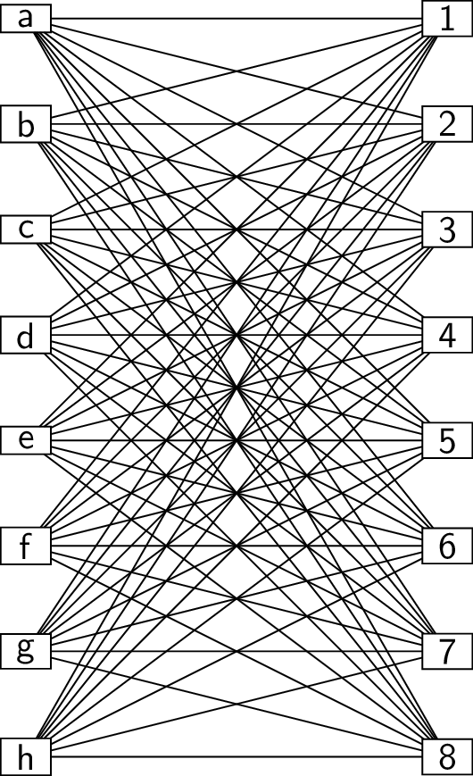
In the rook placement problem, we can take the bipartition \((A,B)\) with \(A
= \{\mathsf a, \mathsf b, \dots, \mathsf h\}\) (the columns of
the chessboard) and \(B = \{\mathsf 1, \mathsf
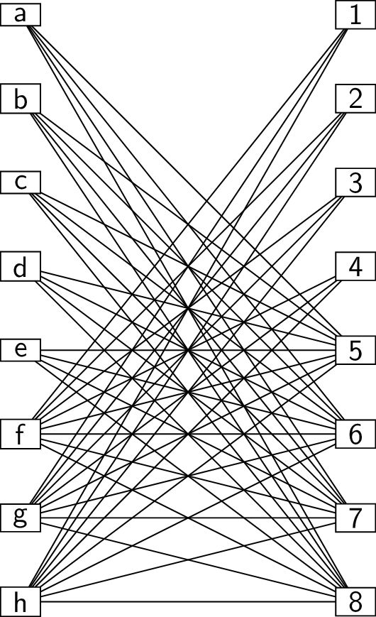
2, \dots, \mathsf 8\}\) (the rows). Figure 13.2 shows the two graphs we get in
this way: Figure 13.2(a) shows the graph for placing
rooks with no restrictions, and Figure 13.2(b)
shows the subgraph when we forbid a \(4\times
5\) rectangle on the board.
As always, we can draw a graph in any way we like; however, when we
want to make it visually clear that a graph is bipartite it is
traditional to arrange the two sides \(A\) and \(B\) in two columns (as in Figure 13.2) or in two rows.
Graph for the entire chessboardSubgraph excluding the forbidden squares
Modeling rook placements with bipartite graphs
The graph in Figure 13.2(a)
representing the entire chessboard is a special case: it is isomorphic
to a complete bipartite graph. (Just as the complete graph has all the
edges a graph could possibly have, a complete bipartite graph has all
the edges a bipartite graph could possibly have.) Here is one general
definition:
Definition 13.2. For any \(m\ge 1\) and \(n\ge 1\), the complete bipartite
graph \(K_{m,n}\) is the graph
with \(m+n\) vertices \(\{1,2,\dots,m+n\}\) and all \(mn\) possible edges \(xy\) where \(1
\le x \le m\) and \(m+1 \le y \le
m+n\).
We have already seen one special case: the star graph \(S_n\) is isomorphic to the complete
bipartite graph \(K_{1,n-1}\).
In the case of the graphs for the rook placement problem, the
bipartition \((A,B)\) is a natural part
of the definition of the graph. The two vertices come in two types,
representing the rows and the columns of the chessboard, and the rule
defining adjacency is a relationship between the two types of
vertex.
It turns out that the grid graph representing the domino problem is
also a bipartite graph. Here, though, the bipartition \((A,B)\) is not given to us. In order to see
that the graph is bipartite, we have to find a pair \((A,B)\) satisfying the definition of a
bipartition.
Can you think of a way to classify the
squares of any chessboard into two types, so that every domino we place
covers one square of each type?
The classification is by color: let \(A\) be the set of light squares and let
\(B\) be the set of dark squares.
The chessboard-style coloring proves that every grid graph \(G(m,n)\) (and every subgraph of a grid
graph) is bipartite. (If we remove opposite corners of the chessboard,
we delete two vertices of the grid graph, but it remains bipartite when
we do so.) Now, let’s talk about how to find the pair \((A,B)\) in general.
A problem that involves labeling the vertices of a graph (such as
with two sides \(A\) and \(B\)) might be difficult because we might
have to guess, make mistakes, and backtrack. In the case of a
bipartition, we are actually quite lucky: there are frequent forced
deductions. In a bipartite graph, if there is an edge \(xy\) where \(x
\in A\), then we know that \(y\in
B\) without guessing. The following algorithm relies only on
making such forced deductions.
Given a graph \(G\), we intend to
give each vertex a label, \(A\) or
\(B\), to indicate which side of the
bipartition it is on. Initially, all vertices start unlabeled.
Pick an arbitrary unlabeled vertex and label it with \(A\).
Go through all vertices newly labeled with \(A\), and label all their neighbors with
\(B\).
Go through all vertices newly labeled with \(B\), and label all their neighbors with
\(A\).
Repeat steps 2–3 until a vertex has been labeled with both \(A\) and \(B\), or until no more unlabeled vertices
are being labeled.
If the graph is not connected, repeat steps 1–4 for each
connected component.
If the graph we are working with is bipartite, then at the end, we
get a bipartition \((A,B)\),
where \(A\) is the set of all vertices
labeled with \(A\), and \(B\) is the set of all vertices labeled with
\(B\).
What happens if the graph is not
bipartite?
We will give a vertex both labels, and
stop. Such a vertex cannot exist in a bipartite graph, so if we are
forced to have such a vertex, then the graph cannot be bipartite.
Why are we free to label a vertex with
\(A\) in step 1: at the beginning, and
when we consider each new connected component?
In each connected component, we can swap
the roles of \(A\) and \(B\). So for every solution where this
vertex is in \(B\), there is another
solution where it is in \(A\).
The bipartition algorithm is quite similar to the distance-finding
algorithm we studied in Chapter 3: in
both algorithms, we visit all the vertices by a breadth-first search.
The only difference is in what we do when we visit the vertices. In the
distance-finding algorithm, we gave a vertex labels \(0, 1, 2, 3, \dots\) at successive stages.
In this algorithm, we alternate the labels \(A, B, A, B, \dots\) at successive stages,
instead.
Let \(G\)
be a connected graph, and let \(x\) be
the vertex initially placed in \(A\).
How can we define the sets \(A\) and
\(B\) in terms of distances from \(x\)?
In the end, \(A\) will be the set of all vertices at an
even distance from \(x\), and \(B\) will be the set of all vertices at an
odd distance from \(x\).
Odd cycles
Although the bipartition algorithm is a convenient way to test a
specific graph for being bipartite, it is not as useful theoretically:
when proving a general result, we would like some testable criteria. One
way to prove a graph is bipartite is to find a bipartition \((A,B)\) and show that it satisfies the
definition, but we’d also like to be able to prove that a graph is not
bipartite. For this, we have the following theorem:
Theorem 13.1. A graph \(G\) is bipartite if and only if it contains
no cycles of odd length (no odd cycles, for short).
We can interpret this theorem as saying that the odd cycle graphs
\(C_3, C_5, C_7, C_9, \dots\) are the
simplest non-bipartite graphs: every other graph that isn’t bipartite
contains one of them.
Proof of Theorem 13.1.
First, we prove that in a bipartite graph, all cycles must have even
length. In fact, we will prove that all closed walks have even length!
The length of a cycle is equal to the length of a walk representing it,
so this will be sufficient.
Let \(G\) be bipartite with
bipartition \((A,B)\), and let \((x_0, x_1, \dots, x_{l-1}, x_0)\) be a
closed walk. Without loss of generality, suppose that \(x_0 \in A\). Because edges \(x_0x_1\), \(x_1x_2\), and so on must have one endpoint
on each side of the bipartition, we must have \(x_1 \in B\), \(x_2 \in A\), and so on. In general, we can
prove by induction that \(x_i \in A\)
whenever \(i\) is even, and \(x_i \in B\) whenever \(i\) is odd: the base case is \(x_0\), and then induction step simply uses
the fact that the endpoints of edge \(x_i
x_{i+1}\) must be on opposite sides.
Since the endpoints of edge \(x_{l-1}x_0\) must be on opposite sides, and
\(x_0 \in A\), we must have \(x_{l-1} \in B\), which means \(l-1\) is odd. Therefore \(l\), the length of the walk, must be even.
The first half of the proof is complete!
It is easy at this point in the proof to get confused and prove the
same thing we just did a second time—for example, this would happen if
we continued by proving that if \(G\)
contains an odd cycle, it is not bipartite. To continue correctly, we
will assume that \(G\) is not
bipartite, and prove that it contains an odd cycle.
The condition “\(G\) is not
bipartite” is very difficult to work with: it says that a bipartition
\((A,B)\) does not exist, or that every
candidate pair \((A,B)\) somehow fails
to be a bipartition. To make use of this, we define a pair \((A,B)\) that ought to be a bipartition in
any bipartite graph. Inspired by our bipartition algorithm, we begin by
choosing a vertex from each connected component of \(G\), and then define:
\(A\) to be the set of all
vertices at an even distance from a chosen vertex;
\(B\) to be the complement of
\(A\): the set of all vertices at an
odd distance from a chosen vertex.
Since \(G\) is not bipartite, this
is not a bipartition. So there must be some edge \(xy\) between two vertices both in \(A\), or both in \(B\). Since \(x\) and \(y\) are necessarily in the same connected
component, they must both be at an even distance, or both at an odd
distance, from the chosen vertex \(z\)
in that component.
Consider the walk that begins at \(x\), follows some shortest \(x-z\) walk, then follows some shortest
\(z-y\) walk, then takes the edge \(xy\). The first two segments of this walk
both have odd length or both have even length, so combined, their length
is even. The final edge \(xy\)
increases the length by \(1\). We’ve
found a closed walk of odd length.
To complete the proof, let \((x_0, x_1,
\dots, x_{l-1}, x_0)\) be a shortest closed walk of odd length:
we will prove that it represents an odd cycle. Suppose not: then there
are some positions \(i\) and \(j\) with \(0\le
i<j < l\) and \(x_i =
x_j\).
The other way the closed walk can fail to
represent a cycle is if \(l<3\). Why
can we rule this out?
Since \(l\) is odd, the only such case is \(l=1\). But a closed walk of length \(1\) cannot exist, because a vertex cannot
be adjacent to itself. (In a multigraph, this would be possible with a
loop, but in a multigraph, the loop would also be an odd cycle.)
The closed walk \((x_i, x_{i+1}, \dots,
x_j)\) has length \(j-i\); the
closed walk \[(x_0, x_1, \dots, x_i, x_{j+1},
x_{j+2}, \dots, x_{l-1}, x_0)\] has length \(l - (j-i)\). Since the sum of these two
lengths is the odd number \(l\), at
least one of these lengths must be odd; since \(i<j<l\), both lengths are smaller
than \(l\). Therefore we’ve found an
even shorter closed walk of odd length, contradicting our initial choice
of a walk. We conclude that the pair \(i,j\) cannot exist: the closed walk we
found does represent an odd cycle! This completes the proof. ◻
In the second half of the proof, why do we
need to laboriously define \(A\) and
\(B\); can we just skip directly to
defining \((x_0, x_1, \dots, x_{l-1},
x_0)\) to be a shortest closed walk of odd length?
Before we can define a shortest closed
walk of odd length, we need to know that the graph contains such closed
walks in the first place: in an empty set of walks, there is no shortest
walk!
To conclude this section, let’s consider two examples of bipartite
graphs, and how we prove that they are bipartite. In one case, we will
use the definition directly; in the other, we will use Theorem 13.1.
Proposition 13.2. For all \(n\ge 1\), the hypercube graph \(Q_n\) is bipartite.
Proof. The vertices of \(Q_n\) are bit strings \(b_1 b_2 \dots b_n\) where each \(b_i\) is either \(0\) or \(1\). To define a bipartition \((A,B)\) of \(V(Q_n)\), we place a vertex \(b_1 b_2 \dots b_n\) in \(A\) if \(b_1 +
b_2 + \dots + b_n\) is even, and in \(B\) if \(b_1 +
b_2 + \dots + b_n\) is odd.
Each edge of \(Q_n\) joins two
vertices \(x\) and \(y\) that differ only in one position; \(x_i \ne y_i\) for some \(i\), but \(x_j =
y_j\) for all \(j\ne i\). As a
result, \[(x_1 + x_2 + \dots + x_n) - (y_1 +
y_2 + \dots + y_n) = x_i - y_i = \pm 1:\] every difference \(x_j - y_j\) with \(j \ne i\) cancels. Since the sums differ by
\(\pm 1\), one of them is even and one
is odd: the edge \(xy\) has one
endpoint in \(A\) and one in \(B\). Therefore \((A,B)\) is a bipartition of \(Q_n\), completing the proof. ◻
What is the relationship between this
bipartition and distances in \(Q_n\)?
This definition places a vertex in \(A\) whenever it is at an even distance from
vertex \(00\dots 0\).
Proposition 13.3. All trees are
bipartite.
Proof. We know from Theorem 10.2
that trees have no cycles at all—in particular, they have no odd cycles,
so they are bipartite by Theorem 13.1. ◻
To discuss problems such as the domino puzzle and the rook puzzle, we
make the following definition.
Definition 13.3. A matching\(M\) in a graph \(G\) is a spanning subgraph of \(G\) in which every vertex has degree \(0\) or \(1\): no two edges in \(E(M)\) share an endpoint.
A vertex \(x \in V(G)\) with \(\deg_M(x) = 1\) is covered
by \(M\), and
uncovered otherwise (when \(\deg_M(x)=0\)). The vertices covered by
\(M\) are exactly the endpoints of the
edges in \(E(M)\).
When it comes to a matching, we are almost exclusively interested in
the edge set \(E(M)\): it tells us
where to place rooks or dominoes. It is common to simply define a
matching to be a set of edges, no two sharing an endpoint. However, the
spanning subgraph \(M\) is occasionally
convenient to use; it is easy to go from \(M\) to \(E(M)\), but not so easy to go from \(E(M)\) back to \(M\), so I have chosen the subgraph and not
the set of edges as the fundamental object.
We can think about matchings in all kinds of graphs. But we will
start by thinking about matchings in bipartite graphs for two reasons.
First, many applications will naturally give us a bipartite graph in
which to look for a matching. Second, the theory turns out to be simpler
for bipartite graphs.
The empty subgraph \(M\) with no
edges is also a matching by our definition—it’s just not a very good
one. It is more difficult, but also more interesting, to select more
edges. The larger a matching is, the more vertices it covers, and so the
absolute limit is to cover every vertex of \(G\): this is what we’re looking for in both
examples we’ve seen so far.
Definition 13.4. A perfect
matching\(M\) in a graph
\(G\) is a matching that covers every
vertex of \(G\).
The bipartite matching problem can be considered from two points of
view. The first is the optimistic point of view, in which we ask whether
a perfect matching exists. This is very common in theoretical
applications, including applications to other areas of math.
There is also what I call the “realistic” point of view. In many
practical applications, while a perfect matching is still the best
option, a very big matching is still good if it is not perfect. For
example, one practical bipartite matching problem occurs in every math
department when instructors are assigned to courses. It might not be
possible in a given semester to offer every course, but does the math
department give up and cancel classes for the semester? No! Instead, the
department simply tries to schedule as many courses as possible.
What bipartite graph can we use to model
assigning instructors to courses?
The vertices of the graph are the course
sections and the instructors that can teach them; the edges represent
which courses an instructor is qualified to teach.
(Further complications on top of the matching problem arise when we
consider giving an instructor multiple sections, which must not be
scheduled at the same time.)
In general, instead of asking whether a perfect matching exists, the
second point of view is to ask how big the largest matchings are. It’s
this point of view that we will start with in this textbook. Of course,
a complete answer to this question will also tell us whether a perfect
matching exists!
Maximum and maximal
In combinatorial optimization problems like the matching problem, we
are trying to find an object \(X\)
that’s as large as possible, subject to some condition. It’s common to
say that \(X\) is:
maximum if it really is as large as you can get; there
are no better solutions than \(X\).
maximal if you cannot add anything to \(X\) without violating the restriction;
there might be better solutions, but you cannot get to them without
removing something from \(X\)
first.
Every maximum solution is also maximal, but the reverse might not
hold.
In the same way, the words minimum and minimal get
used when we’re trying to pick a set that’s as small as possible,
subject to some condition.
In this textbook, I will also use this terminology, but I will avoid
conveying important information solely by the difference between
“maximum” and “maximal”. Usually, we are interested in maximum and
minimum objects, because we want to solve the optimization problems we
pose, and I will let this situation pass by without further comment. If
we really need a maximal object that is not necessarily maximum, or a
minimal object that is not necessarily minimum, I will specifically
point this out for you.
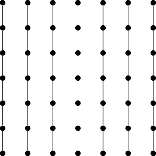
A clumsy packing of dominoes
However, no matter which terminology you use, it’s important to
realize that there is a difference, and in particular there is a
difference in the matching problem. For example, consider the domino
placement in Figure 13.3.
It is not a maximum matching in the \(8\times
8\) grid graph: with no squares removed, it is easy to get a
perfect matching by, for example, placing \(32\) horizontal dominoes. However, it is a
maximal matching: there is no empty space to add another domino.
In fact, in the case of dominoes, a much harder problem is the clumsy
packing problem: what is the minimum number of edges in a maximal
matching of the \(n \times n\) grid
graph? The diagram in Figure 13.3
shows a construction found by Gyárfás, Lehel, and Tuza in 1988 [45].
Looking at this example also tells us that the bipartite matching
problem cannot be solved by a greedy algorithm that selects the first
edges it sees. We should expect to have to work hard before we find a
general solution.
Vertex covers
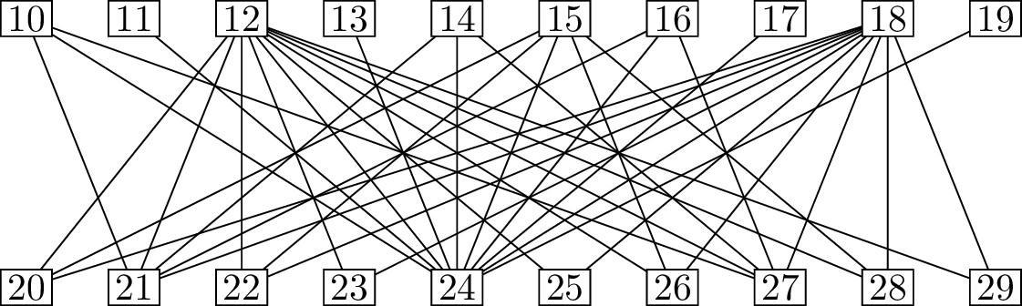
Here is a new, more abstract example of a bipartite matching problem.
Let \(G\) be the bipartite graph with
vertices \(\{10, 11, \dots, 19\}\) on
one side, \(\{20, 21, \dots, 29\}\) on
the other side, and edges defined by the following rule: vertices \(x\) and \(y\) are adjacent when they begin with
different digits and the product \(x \cdot
y\) is divisible by \(6\). A
diagram of the multiples-of-six graph is shown in Figure 13.4, though it is a little
busy in places. What is the largest matching in this graph?
Is there a perfect matching in this
graph?
No: vertices \(11\) and \(13\) on the top are only adjacent to vertex
\(24\), so they cannot both be covered
by a matching.
Look for a matching greedily: for each of
the vertices \(10, 11, \dots, 19\),
match it to the first unused vertex on the other side, if you can. What
matching do you get?
The matching whose edges are \(\{10,21\}\), \(\{11,24\}\), \(\{12,20\}\), \(\{14,27\}\), \(\{15,22\}\), and \(\{18,23\}\).
The multiples-of-six graph
We’ve made a good start, but we have a gap: we’ve found a matching
with \(6\) edges, but we can only prove
that the matching can’t have more than \(9\) edges. (That is, we’ve ruled out a
perfect matching with \(10\) edges.) We
either need to find a better solution, or we need to prove a better
upper bound. Is there a bottleneck—some kind of limited resource that we
exhaust if we try to find a larger matching?
Yes! The limited resource is the vertices divisible by \(3\). To get a product divisible by \(6\), we need both a multiple of \(2\) and a multiple of \(3\), but the multiples of \(3\) are much harder to come by: they are
\(12, 15, 18, 21, 24\), and \(27\). Every edge in a matching needs to use
one of these vertices, so there can be at most \(6\) edges in a matching.
This argument generalizes.
Definition 13.5. A vertex cover
in a graph \(G\) is a set of vertices
\(U\subseteq V(G)\) such that every
edge of \(G\) has one or both endpoints
in \(U\).
For example, in the multiples-of-six graph, the set \(\{12, 15, 18, 21, 24, 27\}\) is a vertex
cover. It is not the only one. For example, the set of all vertices in a
graph is guaranteed to be a vertex cover. The hard task is not to find a
vertex cover, but to find a vertex cover that is as small as
possible.
Vertex covers are important because, just as in the example of the
multiples-of-six graph, we can use them to prove upper bounds on the
size of a matching:
Proposition 13.4. If \(M\) is a matching and \(U\) is a vertex cover in the same graph
\(G\), then \(|E(M)| \le |U|\).
Proof. Consider the sum \[\sum_{x
\in U} \deg_M(u).\] Each term \(\deg_M(x)\) of this sum is at most \(1\), by the definition of a matching, so
the value of the sum is at most \(|U|\): the number of vertices in \(U\).
However, \(\deg_M(u)\) counts the
number of edges of \(M\) incident to
\(x\), so we can also think of the sum
as counting the number of times any edge of \(M\) is incident to any vertex of \(U\). Each edge of \(M\) must be incident to at least one vertex
of \(U\), by the definition of a vertex
cover, so each edge of \(M\)
contributes at least \(1\) to the sum.
Therefore the sum is at least \(|E(M)|\) the number of edges in \(M\).
Putting these inequalities together, we conclude that \(|E(M)| \le |U|\). ◻
In a bipartite graph \(G\), however,
there are two particularly easy examples: if \((A,B)\) is a bipartition of \(G\), then \(A\) and \(B\) are both vertex covers. By
Proposition 13.4, there cannot be a matching
with more than \(\min\{|A|, |B|\}\)
edges; in particular, there can only be a perfect matching if \(|A| = |B|\).
What does this tell us about the domino
problem on an \(8\times 8\) chessboard
with two opposite squares removed?
A complete \(8\times 8\) chessboard has \(32\) squares of each color, but two
opposite squares have the same color; if they are removed, only \(30\) squares of that color are left. So at
most \(30\) dominoes can be placed: not
enough to cover the remaining \(62\)
squares.
Can you use vertex covers to show that the
\(4 \times 5\) rectangle in Figure 13.1(b) cannot be avoided?
Take \(U =
\{\mathsf 5, \mathsf 6, \mathsf 7, \mathsf 8, \mathsf f, \mathsf g,
\mathsf h\}\). These four rows and three columns cover the entire
chessboard except for the highlighted rectangle, showing that at most
\(7\) rooks can be placed outside the
rectangle.
Proposition 13.4 can be used with any matching
\(M\) and any vertex cover \(U\). However, if we want to get upper
bounds on the size of a matching, then the smaller \(U\) is, the better the bounds we get. To
get the best upper bound, we should try to find the smallest vertex
cover possible. However, even for the smallest vertex cover in a graph,
this bound might not tell us the full truth about matchings.
In the complete graph \(K_{100}\), how many edges are in the
largest matching?
There are \(50\), because a \(50\)-edge matching covers all \(100\) vertices: it is perfect.
In the complete graph \(K_{100}\), how many vertices are in the
smallest vertex cover?
There are \(99\). We can leave out any one vertex from
the vertex cover, but a set \(U\)
missing two vertices \(x\) and \(y\) does not contain either endpoint of the
edge \(xy\).
It will turn out that in bipartite graphs, the problems of finding
the largest matching and the smallest vertex cover do “meet in the
middle”. This is a result known as Kőnig’s theorem (Theorem 14.2), which we will prove in the
next chapter. Kőnig’s theorem is the reason we are studying matchings in
bipartite graphs first.
Practice problems
In the graph shown below, find a matching \(M\) and a vertex cover \(U\) with \(|M| =
|U|\).
Mathematicians that study arrangements of non-attacking rooks on
chessboards of various shapes often define an object called the rook
polynomial. This is a polynomial \(p(x)\) in which the coefficient of \(x^k\) is the number of ways to place \(k\) non-attacking rooks onto the
chessboard.
Compute \(a(x)\), the rook polynomial of a \(3\times 3\) chessboard.
Compute \(b(x)\), the rook polynomial of a \(4\times 4\) chessboard.
Prove that the rook polynomial of a \(4\times 4\) chessboard with one square missing is \(b(x) - x \cdot a(x)\).
Prove that the rook polynomial of only the white squares of an ordinary \(8\times 8\) chessboard is \(b(x)^2\).
The “cop-and-highway-robber game”3 is
played on a bipartite graph. One player (the highway robber) chooses an
edge of the graph and occupies it for highway robbery. Simultaneously
and without seeing the edge chosen, the other player (the cop) chooses a
vertex of that edge to guard. If the cop guards an endpoint of the edge
chosen by the highway robber, the highway robber gets caught and loses;
otherwise, the highway robber gets away and wins.
This is a game, like rock-paper-scissors, where both players need to
choose their strategy at random; if either player plays predictably,
then the other player can exploit this.
Suppose that the graph has a matching \(M\). Find a strategy for the highway robber
to win with probability \(1 -
\frac1{|M|}\), no matter what the cop does.
Suppose that the graph has a vertex cover \(U\). Find a strategy for the cop to win
with probability \(\frac1{|U|}\), no
matter what the highway robber does.
Prove that when \(n\) is a
multiple of \(3\), it is possible to
place \(\frac13 n^2\) dominoes on an
\(n \times n\) chessboard so that there
is no more room to place another domino.
Prove that whenever dominoes are placed on an \(n\times n\) chessboard so that there is no
more room to place another domino, at least \(\frac13(n^2 - n)\) dominoes must have been
used.
Prove that a bipartite graph with minimum degree at least \(2\) contains a cycle of length at least
\(4\).
Let \(G\) be a bipartite graph
with bipartition \((A,B)\). Prove the
“bipartite handshake lemma”: \[\sum_{x \in A}
\deg(x) = \sum_{x \in B} \deg(x) = |E(G)|.\]
Coins are placed on several of the squares on an \(8\times 8\) chessboard (at most one coin
per square). Every row of the chessboard has the same number of coins on
it, but every column of the chessboard has a different number of coins
(possibly \(0\)). How many coins are on
the chessboard?
To explore the difference between maximum and maximal matchings,
consider the following graph (which can be made arbitrarily large):
Find a perfect matching in this graph.
Find the smallest matching in this graph above which is maximal
(there is no larger matching that contains all of its edges).
Let \(G\) be a graph (not
necessarily bipartite) and let \(M\) be
a maximal matching in \(G\). Prove that
\(G\) has a vertex cover \(U\) with \(|U| =
2|E(M)|\).
Prove that the graph in this problem is “as bad as it gets”: there is no graph \(G\) with a maximal matching \(M\) and a second matching with more than \(2|E(M)|\) edges.
(BMO 2005) The equilateral triangle \(ABC\) has sides of integer length \(n\). The triangle is completely divided (by
drawing lines parallel to the sides of the triangle) into equilateral
triangular cells of side length 1.
A continuous route is chosen, starting inside the cell with vertex
\(A\) and always crossing from one cell
to another through an edge shared by the two cells. No cell is visited
more than once. Find, with proof, the greatest number of cells which can
be visited.
(Putnam 2025) Alice and Bob play a game with a string of \(n\) digits, each of which is restricted to be \(0\), \(1\), or \(2\). Initially all the digits are \(0\). A legal move is to add or subtract \(1\) from one digit to create a new string that has not appeared before. A player with no legal move loses, and the other player wins. Alice goes first, and the players alternate moves. For each \(n \ge 1\), determine which player has a strategy that guarantees winning.
Footnotes
In the same “rank” or “file”, if you’re a chess
purist.↩︎
In graph theory literature, these have no consistent
name; they can also be called “parts”, or “blocks”, or even “partite
sets”.↩︎
Whose name I made up, inspired by the study of
cops-and-robbers games on graphs, which are something fancier.↩︎