Most chapters in this book are all about giving you tools to deal
with any graph you encounter. This chapter has a bit of that, but it is
much more about showing you examples of some particular useful
graphs.
In Theorem 5.1, we use circulant graphs
(which we previously defined in Chapter 2) to construct
examples of regular graphs in every case where it is possible. In the
next section, I attempt to convey some of the variety of possible
regular graphs out there (except, of course, in the cases without much
variety). Next, we meet the Petersen graph, which will appear as an
example or counterexample many times throughout this book: it will be
especially useful to have in our back pocket when we get to Chapter 17 and Chapter 20.
The last section discusses the degree/diameter problem; this problem
is not exclusive to regular graphs, but many of the examples found when
making progress on it are regular. It is also an example of a research
problem in graph theory where the main form of progress on it is in fact
by finding examples.
There is no general way to find examples; otherwise, problems like
the degree/diameter problem would already be solved. However, being
familiar with a wide variety of examples, and knowing what they’re good
for, is valuable when it comes to writing existence proofs. The proof of
Theorem 5.1 would have been much harder
if we did not already have circulant graphs at our disposal.
In this chapter, we take our first serious look at necessary and
sufficient conditions. This is a theme we will return to throughout the
book; if you need an introduction to necessary and sufficient
conditions, you can find it in Appendix A.
Degree sequences
In Chapter 4, we looked at the degrees of
individual vertices; now, let’s look at all of them together.
Definition 5.1. The degree
sequence of a graph \(G\) is a
sequence of numbers that gives all the degrees of all the vertices of
\(G\).
Despite the word “sequence”, these don’t come in any particular
order, because the vertices of a graph don’t have a particular order.
(There might be a natural order you’re tempted to use based on the way
we drew a graph, but we don’t want the properties of graphs to depend on
how we draw them!) It would have been more reasonable to talk about the
“degree multiset” of a graph: a multiset keeps track of how often its
elements appear, but not their order, which is exactly what we want
here.
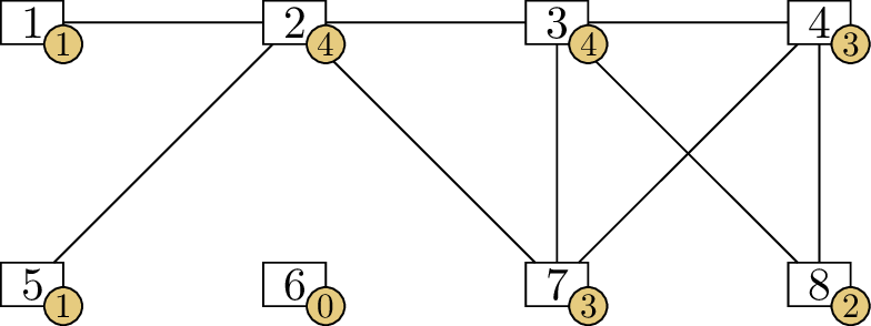
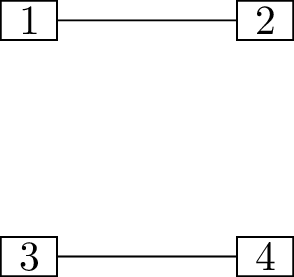
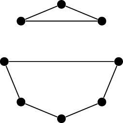
An \(8\)-vertex graph
labeled with the degrees of its vertices
Instead, the convention is to write the degree sequence of a graph in
descending order.1 We do this to avoid the temptation
of looking for meaning in the order of the numbers, and because it will
be convenient for working with the degree sequence. For example, we
would say that Figure 5.1
shows a graph with degree sequence \(4, 4, 3,
3, 2, 1, 1, 0\).
It is a relatively quick and painless process to examine a graph,
count the number of lines poking out of each dot, and in doing so
compute the degree sequence. For this reason, we often look to the
degree sequence first to try to learn about a graph; even if it does not
always tell us what we want to know, it is a quick way to start! This
is, for example, a good way to begin determining whether two graphs are
isomorphic.
If you want to know whether two graphs are
isomorphic, what do their degree sequences tell you?
If \(G\) and \(H\) have different degree sequences,
they’re definitely not isomorphic. If they have the same degree
sequences, they might be isomorphic, but it’s too early to say.
In other words, \(G\) and \(H\) having the same degree sequence is a
necessary condition, but not a sufficient condition for them to be
isomorphic.
Though it is easy to compute the degree sequence of a given graph, it
is harder to go in reverse: to take a sequence of nonnegative integers
in descending order, and determine if it is the degree sequence of some
graph. If it is, we call it a graphic sequence. For
example, \(4, 4, 3, 3, 2, 1, 1, 0\) is
a graphic sequence, and the graph in Figure 5.1 is a proof of this. (There
are other graphs with the same degree sequence, too.)
Here are a few quick puzzles about graphic sequences that illustrate
some things you already know about them, and some things you have yet to
learn.
Problem 5.1. Is the sequence \(8, 8, 8, 8, 8, 8, 8, 8\) graphic?
Answer to Problem 5.1. No: the terms are
too big. This sequence would like to be the degree sequence of an \(8\)-vertex graph, but the largest possible
degree in an \(8\)-vertex graph is
\(7\), achieved when a vertex is
adjacent to all \(7\) other
vertices. ◻
Problem 5.2. Is the sequence \(5, 5, 5, 3, 3, 3, 1, 1, 1\)
graphic?
Answer to Problem 5.2. No: this sequence
violates Corollary 4.2 to the
handshake lemma, which states that a graph cannot have an odd number of
vertices with an odd degree. ◻
Problem 5.3. Is the sequence \(4, 3, 2, 1, 0\) graphic?
Answer to Problem 5.3. No: suppose for
contradiction that \(G\) is a graph
with degree sequence \(4, 3, 2, 1, 0\).
Let \(x\) be the vertex with degree
\(4\) and let \(y\) be the vertex with degree \(0\). Then \(x\) is adjacent to all \(4\) other vertices, so in particular \(xy \in E(G)\); however, \(y\) is adjacent to \(0\) other vertices, so in particular \(xy \notin E(G)\). Therefore it is
impossible for \(G\) to exist. ◻
They give us two rules: in an \(n\)-term graphic sequence, the values must
be integers between \(0\) and \(n-1\), and an even number of them must be
odd.
Are these rules always enough to tell if a
sequence is graphic?
No, and that’s why Problem 5.3 is there. It’s a \(5\)-term sequence in which the values are
integers between \(0\) and \(4\), and \(2\) of them are odd; however, the sequence
is not graphic.
We should think of the rules we deduced from the solutions to
Problem 5.1 and Problem 5.2 as simple preliminary
tests we can carry out before thinking about a sequence very hard. They
are necessary conditions: if a sequence fails one of the two preliminary
tests, it’s definitely not graphic. This can save us a lot of work when
faced with a larger problem of this type.
However, the preliminary tests are not sufficient conditions: if a
sequence passes both preliminary tests, it still might not be graphic.
We will eventually develop a comprehensive theory of graphic sequences,
which will encompass the argument we used to solve Problem 5.3 as a special case.
Regular graphs
As a special case, we can consider the graphic sequence problem for a
sequence in which all terms are equal:
Definition 5.2. A regular graph
is a graph in which every vertex has the same degree. More specifically,
an \(r\)-regular graph
is a graph in which every vertex has degree \(r\). The degree sequence of such a graph is
\(r, r, \dots, r\).
Making a definition does not guarantee that any object satisfying the
definition exists. So when do regular graphs exist?
Suppose the sequence \(r, r, \dots, r\) with \(n\) terms is graphic. What do our two
simple preliminary tests tell us about the relationship between \(r\) and \(n\)?
We must have \(0
\le r \le n-1\), and if \(r\) is
odd, then \(n\) must be even.
In fact, the existence problem for regular graphs is much easier than
the general case. There are no further complications, and these are the
only two conditions.
Theorem 5.1. An \(r\)-regular graph on \(n\) vertices exists whenever \(0 \le r \le n-1\) and at least one of \(r\) or \(n\) is even.
Proof. To prove that an \(r\)-regular graph on \(n\) vertices exists, we need to construct
one.
If we were solving the problem for specific values of \(r\) and \(n\), the proof would be very short: we
could simply draw a diagram and verify that the graph shown has the
right number of vertices, all with the correct degree. To solve the
problem in general, we need to give a family of graphs as the
solution.
Not every family of graphs is sufficiently flexible for our purposes.
For example, in Chapter 4, we defined the family of
hypercube graphs. These are all regular graphs: for any \(r\), if we want an \(r\)-regular graph, the \(r\)-dimensional hypercube graph \(Q_r\) will do. However, there is only one
\(r\)-dimensional hypercube graph, and
it has \(2^r\) vertices. If we want a
regular graph with some other number of vertices, we have to do
something else.
Fortunately, we do have a very flexible family of regular graphs at
our fingertips: the circulant graphs introduced in Chapter 2. These are actually
even more flexible than we need: for large \(n\), we can pick from many examples of
circulant graphs for each possible degree. To remind you of the
definition, the circulant graph \(\operatorname{Ci}_n(d_1, d_2, \dots, d_k)\)
has vertex set \(\{0,1,\dots,n\}\),
which we think of as being arranged around a circle, in that order. Two
vertices \(x\) and \(y\) are adjacent if \(x - y \equiv \pm d_i \pmod n\) for some
\(i\); if \(x\) and \(y\) are \(d_i\) steps apart around the circle.
Usually, each offset \(d_i\) gives
each vertex \(x\) two neighbors: \(x - d_i \bmod n\) and \(x + d_i \bmod n\). As a result, if \(r\) is even, we can get an \(r\)-regular circulant graph by using \(\frac r2\) offsets. To give a concrete
example, \(\operatorname{Ci}_n(1, 2, \dots,
\frac r2)\) will be an \(r\)-regular graph for all even \(r\) between \(2\) and \(n-1\), proving almost half of the theorem
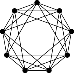
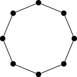
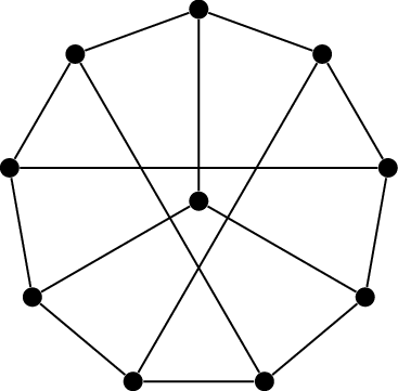
by itself. (For an example, see Figure 5.2(a): this
is the graph we use when \(n=9\) and
\(r=6\).)
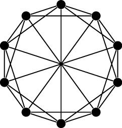
Circulant graphs in the proof of Theorem 5.1What if \(r=0\)?
I am reluctant to write \(\operatorname{Ci}_n()\), because this looks
weird, but it’s true that if we don’t give a circulant graph any
offsets, then there will be no edges: the result is a \(0\)-regular graph, for any positive integer
\(n\).
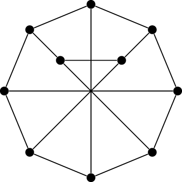
It is a bit trickier to get an \(r\)-regular circulant graph when \(r\) is odd. We know that it is impossible
to find an \(r\)-regular graph on \(n\) vertices if both \(r\) and \(n\) are odd, so we may assume that \(n\) is even. But how does this help us?
In what exceptional case does an offset
\(d_i\) in a circulant graph not
contribute \(+2\) to the degree of
every vertex?
When \(n\) is even and the offset is equal to
\(\frac n2\).
For any \(x\), \(x - \frac n2 \bmod n\) and \(x + \frac n2 \bmod n\) are the same vertex:
if we think of the vertices as being arranged around a circle, then this
is the vertex opposite \(x\). So
including the offset \(\frac n2\) lets
us obtain an \(r\)-regular graph when
\(r\) is odd. Again, we must give a
concrete example to make the proof precise about it does, so let our
example be \(\operatorname{Ci}_n(1, 2, \dots,
\frac{r-1}{2}, \frac n2)\). (For an example, see Figure 5.2(b): this is the graph we use when
\(n=10\) and \(r=5\).)
Why is this an \(r\)-regular graph?
For each \(i=1,
\dots, \frac{r-1}{2}\), a vertex \(x\) is adjacent to \(x + i \bmod n\) and \(x - i \bmod n\), giving it \(2 \cdot \frac{r-1}{2}\) or \(r-1\) neighbors. The last neighbor is \(x + \frac n2 \bmod n\).
Because \(r \le n-1\), it is always
true that \(\frac{r-1}{2} < \frac
n2\), so the initial progression \(1,
2, \dots, \frac{r-1}{2}\) never risks overlapping the exceptional
case \(r = n\). Similarly, in our
previous case when \(r\) was even, the
offsets \(1, 2, \dots, \frac r2\) never
included the “exceptional” offset \(\frac
n2\), because \(\frac r2 < \frac
n2\).
This completes the proof: for all \(r\) and \(n\) such that \(0
\le r \le n-1\) and at least one of \(r\) or \(n\) is even, either the circulant graph
\(\operatorname{Ci}_n(1, 2, \dots, \frac
r2)\) (for even \(r\)) or the
circulant graph \(\operatorname{Ci}_n(1, 2,
\dots, \frac{r-1}{2}, \frac n2)\) (for odd \(r\)) is an \(r\)-regular graph on \(n\) vertices. ◻
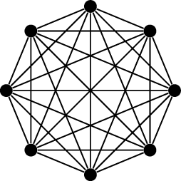
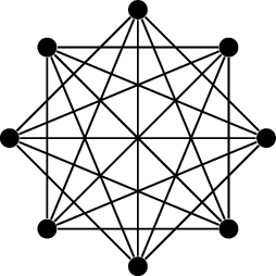
What graph do we end up constructing when
\(r=n-1\)?
For odd \(n\), we get \(\operatorname{Ci}_n(1,2,\dots,\frac{n-1}{2})\),
and for even \(n\), we get \(\operatorname{Ci}_n(1,2,\dots,\frac n2)\),
but in both cases, the result is isomorphic to the complete graph \(K_n\). This is because in both cases, we’ve
included every possible offset. For an example of this, see Figure 5.2(c).
I chose the circulant graphs I did in the proof of Theorem 5.1 not just because they’re the
simplest possible choice, but for another reason. The \(r\)-regular circulant graph on \(n\) vertices that we used has a special
name: the Harary graph, denoted \(H_{n,r}\). For example, the graphs in
Figure 5.2 are \(H_{9,6}\) (Figure 5.2(a)),
\(H_{10,5}\) (Figure 5.2(b)), and \(H_{8,7}\) (Figure 5.2(c)).
We will see these graphs again in Chapter 26, where we will
put them to the same use as their inventor Frank Harary did in
1962 [49]: as examples
of graphs of a given connectivity with as few edges as possible.
How many regular graphs are
there?
Though Theorem 5.1
proves the existence of \(r\)-regular,
\(n\)-vertex graphs with all compatible
values of \(n\) and \(r\), we’ve only found one graph for each
pair \((n,r)\). How many possibilities
exist in total? Let’s start with some small values of \(r\) and see how the story unfolds.
When \(r=0\), every vertex is an
isolated vertex: it has degree \(0\).
There cannot be any edges. For any possible vertex set, there is exactly
one graph, sometimes called the empty graph.
When \(r=1\), whether we believe in
one possibility or multiple possibilities depends on how we count. You
see, suppose \(x\) is a vertex in a
\(1\)-regular graph. Then \(x\) has only one neighbor, which we can
call \(y\). Vertex \(y\) also has only one neighbor, and we
already know what it is: \(x\). Thus,
\(x\) and \(y\) form a \(2\)-vertex connected component with each
other and nothing else, and the entire graph is split up into \(n/2\) such components. (A \(1\)-regular graph, as we already know, is
only possible when \(n\) is even, so
\(n/2\) is an integer.)
The counting difficulty comes in when we ask how many ways there are
to choose these components. In one sense, there are many options:
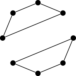
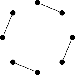
Figure 5.3 shows three different
possibilities in just the \(4\)-vertex
case, and the total number of possibilities grows quickly. However, they
are all isomorphic to each other. We say that there are \(3\) different \(1\)-regular graphs with vertex set \(\{1,2,3,4\}\), but that up to isomorphism,
there is only one \(1\)-regular graph
with \(4\) vertices. This is a term
we’ll use often, so let me give it a formal definition:
Definition 5.3. A description of a graph \(G\)up to isomorphism is a
description which is not necessarily true of \(G\), but is true of some graph isomorphic
to \(G\).
Here are some of the ways this phrase is used, in other
circumstances.
We say that the solution to a problem is unique up to isomorphism
when all solutions to the problem are isomorphic graphs.
We say that \(S\) is the set of
all graphs of some type, up to isomorphism, when every graph of that
type is isomorphic to some graph in \(S\), and no two graphs in \(S\) are isomorphic. If \(|S|=k\), we might also say that there are
\(k\) graphs of that type, up to
isomorphism.
We say that the result of an operation is some particular graph
\(G\), up to isomorphism, if the
operation results in a graph isomorphic to \(G\), but possibly not with the same vertex
set as \(G\).
Statements up to isomorphism are also sometimes phrased in terms of
unlabeled graphs, which is a perspective I’ll say more about in
Chapter 11, but I prefer to avoid it,
because it causes more confusion. For any graph \(G\), the vertex set \(V(G)\) is a set of distinguishable objects,
whether or not we distinguish them in a diagram of \(G\).
Three different(?) \(1\)-regular graphs with vertex set \(\{1,2,3,4\}\)
Moving on, let’s consider what happens when \(r=2\). The example we constructed in
Theorem 5.1 is \(\operatorname{Ci}_n(1)\), but this is
isomorphic to a more common graph: the cycle graph \(C_n\). This is also unique in a sense, but
a slightly different sense:
Proposition 5.2. Up to isomorphism, \(C_n\) is the unique connected \(2\)-regular graph with \(n\) vertices.
Proof. First of all, we check that \(C_n\) a connected \(2\)-regular graph. In \(C_n\) (with vertex set \(\{1,2,\dots,n\}\)) vertex \(x\) is adjacent to \(x-1\) and \(x+1\), treating \(1-1\) as \(n\) and \(n+1\) as \(1\), so \(\deg(x)
= 2\) for all \(x \in V(C_n)\).
For all \(x,y \in V(C_n)\), the
sequence \((x,x+1,\dots,y)\) is an
\(x-y\) walk if \(x<y\), and the sequence \((x,x-1,\dots,y)\) is an \(x-y\) walk if \(x>y\); this makes \(C_n\) connected.
Next, let \(G\) be an arbitrary
connected \(2\)-regular graph. Then in
particular \(G\) has minimum degree
\(2\), so Theorem 4.4 applies
and tells us that \(G\) contains a
cycle \(C\). For all \(x \in V(C)\), we know \(\deg_C(x) = 2\) because \(C\) is a cycle, and \(\deg_G(x) = 2\) because \(G\) is \(2\)-regular, so \(x\) has no neighbors in \(G\) other than the two it has in \(C\). There are no edges with exactly one
endpoint in \(V(C)\), so by Lemma 3.2, either
\(G = C\) or else \(G\) wouldn’t be the connected graph we took
it to be. But \(G = C\) makes \(G\) isomorphic to a cycle graph, completing
our proof. ◻
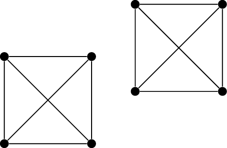
\(C_8\)Two copies of \(C_4\)Copies of \(C_3\) and \(C_5\)
Three non-isomorphic \(2\)-regular graphs with \(8\) vertices
The difference between the \(1\)-regular and \(2\)-regular case is that we can obtain more
examples by taking graphs with multiple connected components. Each
component, by Proposition 5.2, is a cycle; we can
mix and match cycles however we like to reach a total of \(n\) vertices. Figure 5.4 shows three
non-isomorphic possibilities for an \(8\)-vertex \(2\)-regular graph: it could be isomorphic
to \(C_8\) (Figure 5.4(a)), or to the union of two
copies of \(C_4\) (Figure 5.4(b)), or to the union of copies
of \(C_3\) and \(C_5\) (Figure 5.4(c)).
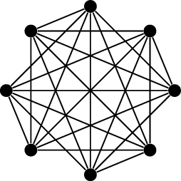
Once \(r \ge 3\), any hope of
classifying the \(r\)-regular graphs on
\(n\) vertices goes out the window.
Even when \(r=3\), there are many
examples.
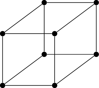
\(Q_3\)Two copies of \(K_4\)The Frucht graph
Three examples of \(3\)-regular graphs
Figure 5.5 shows several \(3\)-regular graphs. You will recognize the
graph in Figure 5.5(a): it is the cube graph \(Q_3\). The graph in Figure 5.5(b) should not be too much of a
surprise either: it is the disjoint union of two copies of \(K_4\), and is the smallest \(3\)-regular graph that is not
connected.
You might be forgiven for thinking, based on the examples you’ve
seen, that regular graphs are highly symmetric—after all, every vertex
has the same degree, which makes every vertex like every other, at least
superficially. To dissuade you from that impression, I’ve included a
final example in Figure 5.5(c): the Frucht graph. It is named
after Robert Frucht, who discovered it in 1949 [35]. The Frucht graph is notable for being
completely asymmetric; in other words, it has no automorphisms, other
than the identity automorphism!
The Frucht graph is just the smallest graph with this property. When
\(n\) is large, it is very rare for a
\(3\)-regular graph with \(n\) vertices to have a nontrivial
automorphism. Don’t be misled by graphs like circulant graphs, which
have a lot of symmetry—they are just the graphs it is easiest to point
to, precisely for that reason. (Think about how much effort it would be
to describe the Frucht graph exactly, compared to how easy it is to
define the circulant graph \(\operatorname{Ci}_{12}(1,6)\), which has
the same number of vertices and edges.)
The Online Encyclopedia of Integer Sequences (OEIS) lists integer
sequences with notable mathematical properties. Entry A002851 of the
OEIS [80] gives the
number of connected \(3\)-regular
graphs on \(2n\) vertices, up to
isomorphism. I cite an online encyclopedia rather than give a formula
because there is no clean formula for the entries of this sequence.
However, you can observe that they grow rather quickly from the first
few entries. Starting from \(2n = 4\),
the sequence is \[1, 2, 5, 19, 85, 509, 4060,
41301, 510489, 7319447, \dots\]
You can probably guess that the story for \(4\)-regular graphs, \(5\)-regular graphs, and so on is very
similar. We only regain any semblance of order once \(r\) gets very close to \(n\). We discover that semblance of order by
taking the complement graph: toggling all the edges from present to
absent and vice versa.
If \(G\)
is an \(r\)-regular graph on \(n\) vertices, what can you say about the
degrees in its complement \(\overline
G\)?
Every vertex \(x
\in V(G)\) has \(r\) neighbors
in \(G\), out of \(n-1\) other vertices, so its neighbors in
\(\overline G\) are the \((n-1)-r\) vertices it was not previously
adjacent to. Therefore \(\overline G\)
is \((n-r-1)\)-regular.
Figure 5.6 shows some examples of
regular graphs and their complements. For example, the cycle graph \(C_8\) is an \(8\)-vertex \(2\)-regular graph we understand, so we must
also be able to understand its complement, an \(8\)-vertex \(5\)-regular graph. We already understand
the complete graph \(K_n\) quite well;
it is the only \(n\)-vertex \((n-1)\)-regular graph, up to isomorphism,
becuase if every vertex has degree \(n-1\), then it is adjacent to all \(n-1\) other vertices. In fact, the empty
graph we previously took as our \(0\)-regular example is commonly written
\(\overline{K_n}\), taking the complete
graph as a starting point.
Up to isomorphism, there is only one \(1\)-regular graph on \(n\) vertices, and only when \(n\) is even. Taking its complement, we
learn that up to isomorphism, there is only one \((n-2)\)-regular graph on \(n\) vertices, and only when \(n\) is even. Figure 5.6(c) and Figure 5.6(d) show an example of
this.
Among \(2\)-regular graphs, cycles
are special; they are the only connected graphs. Among \((n-3)\)-regular graphs, the complements of
cycles are not as special, because (for \(n\ge
5\)) all \((n-3)\)-regular
graphs are connected. Still, by taking the complement of every graph in
Figure 5.4, we could find all the
\(5\)-regular \(8\)-vertex graphs, up to isomorphism; the
same strategy works for all \(n\).
The Petersen graph
Having seen a bit of the variety of regular graphs out there, we’ll
now look at another useful family of regular graphs. We’ll begin with a
specific example, known as the Petersen graph after its discoverer,
Julius Petersen.
The Petersen graph is notable in graph theory for many reasons. In
this textbook, we will see it several times in its role of providing a
small counterexample to several plausible-sounding conjectures in graph
theory. There are also several classification theorems (which we will
not see) in which it plays a central role. Entire books [57] have been written about
this graph.
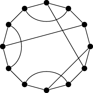
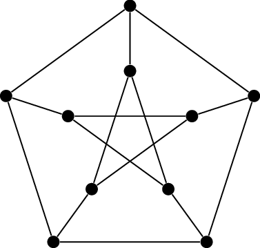
Three diagrams of the Petersen graph
Three diagrams of the Petersen graph are shown in Figure 5.7, showing some of the
symmetry it has: one with \(5\)-fold
rotational symmetry, one with \(3\)-fold symmetry, and one which nearly has
\(4\)-fold symmetry (but not quite). In
fact, the Petersen graph is much more symmetric than any of these
diagrams show, which can be seen from its combinatorial definition:
Definition 5.4. The Petersen
graph is the graph with vertex set \[\{12, 13, 14, 15, 23, 24, 25, 34, 35,
45\}\] consisting of all unordered pairs of elements of \(\{1,2,3,4,5\}\), and an edge between two
vertices whenever they have no elements of \(\{1,2,3,4,5\}\) in common. (For example,
vertex \(12\) is adjacent to vertices
\(34\), \(35\), and \(45\).)
This definition has a much greater degree of symmetry than either of
the diagrams! For any permutation of the set \(\{1,2,3,4,5\}\), we can relabel the
vertices of the Petersen graph according to that permutation; this will
not change which vertices have no elements of \(\{1,2,3,4,5\}\) in common, so it is an
automorphism of the Petersen graph. All \(5! =
120\) automorphisms of the Petersen graph can be described in
this way.
The Petersen graph is part of an infinite family of regular, highly
symmetric graphs known as the Kneser graphs. For all integers \(n\) and \(k\) with \(0 \le
k \le n\), the vertices of the Kneser graph \(K(n,k)\) are the \(k\)-element subsets of the set \(\{1,2,\dots,n\}\). As in the definition of
the Petersen graph, two vertices of \(K(n,k)\) are adjacent if they have no
elements in common. (The definition is only interesting when \(n \ge 2k\); otherwise, any two \(k\)-element subsets of \(\{1,2,\dots,n\}\) are guaranteed to
overlap.)
How many vertices does \(K(n,k)\) have, as a function of \(n\) and \(k\)?
There are \(\binom nk\) vertices: the number of ways to
choose \(k\) unordered elements of
\(\{1,2,\dots,n\}\) without
repetition.
What is the degree of an arbitrary vertex
of \(K(n,k)\)?
A vertex \(X\) has \(\binom{n-k}{k}\) neighbors: the \(k\)-element subsets of the set \(\{1,2,\dots,n\} - X\).
This explains why the Kneser graphs are always regular. For the same
reason as the Petersen graph, they have many automorphisms. Though the
Petersen graph is by far the most widely encountered of the Kneser
graphs, they all have applications to the combinatorics of set families,
due to their definition via subsets of \(\{1,2,\dots,n\}\).
For now (in this section), I will prove only one property of the
Petersen graph, which might look silly on its own. However, it will be a
starting point for other proofs, and in the next section, we will see
one example of how it can be useful. This lemma is also a good example
of how to use symmetry in a proof.
Lemma 5.3. The Petersen graph has no cycles of
length \(3\) or \(4\).
Proof. To check such a claim with as little effort as
possible, it helps to make use of the many automorphisms of the Petersen
graph. Take any two adjacent vertices of the Petersen graph: these are
unordered pairs \(ab\) and \(cd\), where \(a,b,c,d\) are four distinct elements of
\(\{1,2,3,4,5\}\). Then there is an
automorphism of the Petersen graph that relabels \(a\) to \(1\), \(b\)
to \(2\), \(c\) to \(3\), and \(d\) to \(4\) in every vertex, taking our two
adjacent vertices to \(12\) and \(34\).
How do we use this? Well, suppose \(C\) is an arbitrary cycle in the Petersen
graph, and \(ab\) and \(cd\) are two vertices adjacent in \(C\). By applying the automorphism above to
\(C\), we get a new cycle \(C'\) in the Petersen graph on which
\(12\) and \(34\) are two consecutive vertices. The
automorphism is a bijection, so \(C\)
and \(C'\) have the same number of
vertices: if we prove \(C'\) has
length at least \(5\), we conclude that
\(C\) has length at least \(5\).
(When writing for an audience familiar with such tricks, it is common
to simply say: “Let \(C\) be a cycle in
the Petersen graph. By symmetry, we may assume that \(12\) and \(34\) are two consecutive vertices along
\(C\).” The proof becomes much
shorter.)
On a cycle of length \(3\), two
consecutive vertices have a common neighbor: the third vertex. On a
cycle of length \(4\), two consecutive
vertices each have another neighbor, and those two neighbors must
themselves be adjacent. To complete the proof, we show that neither of
these scenarios is possible in the Petersen graph, when \(12\) and \(34\) are the two consecutive vertices.
The other neighbors of \(12\) are
\(35\) and \(45\); the other neighbors of \(34\) are \(15\) and \(25\). From this we can see that \(12\) and \(34\) have no common neighbors, so our cycle
cannot have length \(3\); also, none of
the neighbors of \(12\) and \(34\) are adjacent (all of them include the
number \(5\)), so our cycle cannot have
length \(4\). ◻
The degree/diameter problem
In Chapter 3, we defined the distance \(d_G(x,y)\) between two vertices in a graph
\(G\) to be the minimum length of an
\(x-y\) walk in \(G\). A related concept is the
diameter of \(G\): the largest
distance between any pair of vertices.2
That is, a graph has diameter \(D\) if
we can reach every vertex from every other vertex in at most \(D\) steps, but there are some cases in
which we cannot do it in fewer than \(D\) steps.
It’s worth pointing out that the diameter is defined by a
maximization problem (it is the largest distance) with a minimization
problem inside it (the distance is the smallest possible length of a
walk). This means that proving that the diameter of a graph has a
certain value takes some getting used to: it is a mix of specific
examples and universal bounds, in both directions.
How might you prove that a graph \(G\) has diameter at least \(D\)?
By proving that \(d_G(x,y) \ge D\) for two particular
vertices \(x\) and \(y\): showing that there are no \(x-y\) walks of any length less than \(D\).
How might you prove that a graph \(G\) has diameter at most \(D\)?
By proving that \(d_G(x,y) \le D\) for all pairs of vertices
\(x,y\), showing that we can get from
every vertex to every other in at most \(D\) steps.
We can see both kinds of proof in action when we prove the following
result, which is also the first noteworthy use of the Petersen graph in
this textbook.
Proposition 5.4. Among all graphs with maximum
degree \(3\) and diameter \(2\), the Petersen graph has the most
vertices.
Proof. First, we should verify that the Petersen graph
actually does have diameter \(2\). The
lower bound is quick: a diameter of \(1\) would mean that all vertices are
adjacent, and the Petersen graph certainly has pairs of vertices that
are not adjacent (such as \(12\) and
\(13\)). Therefore the Petersen graph
has diameter at least \(2\).
For the upper bound, we must show that no matter which vertex \(x\) we choose in the Petersen graph, all
vertices are within distance \(2\) of
\(x\). Since the Petersen graph is
\(3\)-regular, \(x\) has three neighbors; call them \(y_1, y_2, y_3\). Each \(y_i\) has two neighbors other than \(x\). By Lemma 5.3, \(y_i\) cannot be adjacent to another \(y_j\) (or else \((x,y_i,y_j,x)\) would represent a cycle of
length \(3\)), and two neighbors \(y_i\) and \(y_j\) of \(x\) cannot have a common neighbor \(z\) (or else \((x,y_i,z,y_j,x)\) would represent a cycle
of length \(4\).) Therefore there are
six different vertices \(z_1, \dots,
z_6\) all adjacent to a neighbor of \(x\).
Altogether, we’ve named \(10\)
vertices: \(x\), \(y_1, \dots, y_3\), and \(z_1, \dots, z_6\). All are different, and
all are within distance \(2\) of \(x\). But the Petersen graph only has \(10\) vertices, so we conclude that all
vertices are within distance \(2\) of
\(x\). Since \(x\) was arbitrary, the diameter of the
Petersen graph is at most \(2\).
The last part of the proof is the interesting part, in my opinion. We
must prove that a graph \(G\) with
maximum degree \(3\) and diameter \(2\) can have at most \(10\) vertices: the number of vertices in
the Petersen graph. In such a graph, if we pick an arbitrary vertex
\(x\), we can write \(V(G)\) as \(\{x\}
\cup Y \cup Z\), where \(Y\) is
the set of vertices at distance \(1\)
from \(x\), and \(Z\) is the set of vertices at distance
\(2\) from \(x\).
The graph \(G\) has maximum degree
\(3\), so in particular, \(x\) has at most \(3\) neighbors; every vertex in \(Y\) must be a neighbor of \(x\), so \(|Y| \le
3\). Meanwhile, for every vertex \(z
\in Z\), there is a path \((x,y,z)\) of length \(2\); here, \(y
\in Y\), because it is adjacent to \(x\). Each vertex has at most \(3\) neighbors, but one of them is \(x\): it has at most \(2\) neighbors in \(Z\). Together, the vertices in \(Y\) have at most \(3 \cdot 2 = 6\) neighbors in \(Z\), but each vertex in \(Z\) must have a neighbor in \(Y\): so \(|Z|=6\).
Putting this together, \(|V(G)| = |\{x\}| +
|Y| + |Z| \le 1 + 3 + 6 = 10\), so \(G\) can have at most \(10\) vertices. The Petersen graph, with
\(10\) vertices, is optimal. ◻
The degree/diameter problem studies the generalization of
Proposition 5.4: for a pair of positive
integers \((\Delta,D)\), what is the
largest number of vertices in a graph with maximum degree \(\Delta\) and diameter \(D\)?
Theorem 5.5. A graph \(G\) with maximum degree \(\Delta \ge 2\) and diameter \(D\) can have at most \[1 + \Delta + \Delta(\Delta-1) +
\Delta(\Delta-1)^2 + \dots + \Delta(\Delta-1)^{D-1}\] vertices,
which is \(2D+1\) if \(\Delta=2\) and \(1 + \Delta \frac{(\Delta-1)^D - 1}{\Delta -
2}\) if \(\Delta >
2\).
Proof. As in the proof of Proposition 5.4, we pick an arbitrary
vertex \(x\) and write the vertex set
of \(G\) as \[V(G) = Y_0 \cup Y_1 \cup Y_2 \cup \dots \cup
Y_D\] where \(Y_0 = \{x\}\) and
\(Y_i\) is the set of all vertices at
distance \(i\) from \(x\).
Next, by induction on \(i\), we show
that \(|Y_i| \le
\Delta(\Delta-1)^{i-1}\) for \(1 \le i
\le D\). When \(i=1\), this
inequality says that \(|Y_1| \le
\Delta\), which is true because \(x\) has at most \(\Delta\) neighbors, and every vertex in
\(Y_1\) is a neighbor of \(x\). This proves the base case.
An important property we’ll need before we continue is that for \(1 \le i \le D\), a vertex \(y \in Y_i\) must have a neighbor in \(Y_{i-1}\). That’s because there is an \(x-y\) walk of length \(i\) in \(G\). Let \(z\) be the next-to-last vertex on that
walk: the walk is \((x, \dots, z, y)\).
This \(z\) will be the neighbor of
\(y\) in \(Y_{i-1}\).
Why is \(z\) a neighbor of \(y\)?
By the definition of a walk, \(yz\) must be an edge.
Why is there an \(x-z\) walk of length \(i-1\)?
Remove the last vertex \(y\) from the walk \((x,\dots, z,y)\) to get such an \(x-z\) walk.
Why is there no \(x-z\) walk of length \(i-2\) or less?
We could take such a walk and add \(y\) to the end, getting an \(x-y\) walk of length \(i-1\) or less; this contradicts \(y \in Y_i\).
Now we’re ready for the induction step. Suppose that for \(1 \le i \le D-1\), we have already shown
that \(|Y_i| \le
\Delta(\Delta-1)^{i-1}\), and want to move on to \(|Y_{i+1}|\). Each vertex in \(Y_i\) has at least one neighbor in \(Y_{i-1}\), so it has at most \(\Delta-1\) neighbors in \(Y_{i+1}\). Together, there are at most
\(\Delta(\Delta-1)^{i-1}\) vertices in
\(Y_i\), so they have at most \(\Delta(\Delta-1)^i\) neighbors in \(Y_{i+1}\). But every vertex in \(Y_{i+1}\) must be such a neighbor, so \(|Y_{i+1}| \le \Delta(\Delta-1)^i\),
completing the induction step.
Once the induction is concluded, we have \[\begin{aligned}
|V(G)| &= |Y_0| + |Y_1| + |Y_2| + \dots + |Y_D| \\
&= 1 + \underbrace{\Delta}_{|Y_1|} +
\underbrace{\Delta(\Delta-1)}_{|Y_2|} +
\underbrace{\Delta(\Delta-1)^2}_{|Y_3|} + \dots +
\underbrace{\Delta(\Delta-1)^{D-1}}_{|Y_D|},
\end{aligned}\] which is exactly the bound we wanted. When \(\Delta=2\), the bound on \(|Y_i|\) simplifies to \(2\) for every \(i\), giving us \(2D+1\) for the sum. When \(\Delta > 2\), the formula \(1 + \Delta \frac{(\Delta-1)^D - 1}{\Delta -
2}\) comes from the formula for the sum of a finite geometric
series: \(a + ar + ar^2 + \dots + ar^n = a
\frac{r^{n+1}-1}{r-1}\). ◻
The upper bound in Theorem 5.5 is
called the Moore bound after Edward Moore (the same Moore that
discovered the distance-finding algorithm discussed in Chapter 3). Moore also posed the problem
of finding the graphs which achieve the bound exactly, and such graphs
are known as Moore graphs. For example, Proposition 5.4 tells us that the
Petersen graph is a Moore graph. In order for the inequalities of
Theorem 5.5 to be equations, Moore graphs
must all be regular graphs: the maximum degree \(\Delta\) must actually be the degree of
every vertex.
Moore graphs are very rare, apart from a few initial cases: they
exist for all \(\Delta \ge 2\) when
\(D=1\), and for all \(D\ge 1\) when \(\Delta=2\). I will leave it to you, in the
practice problems, to understand these two constructions. Moore graphs
were first studied by Alan Hoffman and Robert Singleton in 1960 [56], who found the Petersen
graph for \((\Delta,D) = (3,2)\) and a
graph called the Hoffman–Singleton graph for \((\Delta,D) = (7,2)\). What’s more, they
proved that when \(D=2\) or \(D=3\), and \(\Delta \ge 3\), there are no more Moore
graphs—with one possible exception. Hoffman and Singleton were unable to
determine if there is a Moore graph with \(\Delta=57\) and \(D=2\); to this day, we do not know the
answer!
Since 1960, the degree/diameter problem has advanced considerably; a
2013 survey by Mirka Miller and Jozef Širáň [73] summarizes much of the recent progress. We
now know that, aside from the two graphs found by Hoffman and Singleton,
and the possible \((\Delta,D) =
(57,2)\) case, there are no Moore graphs with \(\Delta \ge 3\) and \(D\ge 2\). In most cases, the best
constructions we know are very far from the upper bound of Theorem 5.5. Many, but not all of them are
regular graphs.
Practice problems
What are the possible values of the diameter of an \(8\)-vertex graph? Give an example for each
possible value.
If \(n\) and \(r\) are both odd, then an \(r\)-regular graph on \(n\) vertices does not exist, but a Harary
graph \(H_{n,r}\) still does. In this
case, \(H_{n,r}\) is a nearly-regular
graph: it is a graph on \(n\) vertices
where \(n-1\) of them have degree \(r\), and one has degree \(r+1\).
It is defined starting from the Harary graph \(H_{n,r-1}\), or \(\operatorname{Ci}_n(1,2,\dots,\frac{r-1}{2})\).
To this graph, we add \(r+1\) edges
that increase the degree of vertex \(0\) by \(2\), and the degree of vertices \(1, 2, \dots, n-1\) by \(1\) each.
How can we do this? Prove that your method works in general.
Here is a fragment of an alternate proof of the \(r=3\) case of Theorem 5.1.
…assume that a \(3\)-regular
graph \(H\) on \(n-4\) vertices exists. Then, we can create
a \(3\)-regular graph \(G\) on \(n\) vertices, just by adding a new
connected component to \(H\): four new
vertices adjacent to each other and to no other vertices …
What kind of a proof is this? What else do we need to do to finish
the proof of Theorem 5.1
using this idea?
For each diagram in Figure 5.7,
show how to label the vertices with elements of the set \(\{12, 13, \dots, 45\}\) (the vertex set of
the Petersen graph) so that two vertices are adjacent in the diagram if
and only if their labels have no digit in common.
Prove that for all \(n \ge 5\),
the complement of the path graph \(P_n\) has diameter \(2\).
Prove that the Kneser graph \(K(n,k)\) is connected when \(n > 2k\).
Find and prove a similar condition that determines when \(K(n,k)\) has diameter \(2\).
Find and prove a similar condition that determines when \(K(n,k)\) has no cycles of length \(3\) or \(4\).
For all \(\Delta \ge 2\), there
is a Moore graph with maximum degree \(\Delta\) and diameter \(1\) (and \(\Delta+1\) vertices). What is it?
For all \(D\ge 1\), there is a
Moore graph with maximum degree \(2\)
and diameter \(D\) (and \(2D+1\) vertices). What is it?
Prove that, just like the Petersen graph, the Hoffman–Singleton
graph has no cycles of length \(3\) or
\(4\). (You do not know very much about
the Hoffman–Singleton graph, but all you need to know for this problem
is there in this chapter.)
Let \(\Delta \ge 3\). Prove that
if a graph \(G\) with maximum degree
\(\Delta \ge 2\) and diameter \(D\) is not regular, then it has at most
\[1 + (\Delta-1) + (\Delta-1)^2 + \dots +
(\Delta-1)^{D-1} = \frac{(\Delta-1)^D + 1}{\Delta-2}\] vertices:
approximately \(\frac{\Delta-1}{\Delta}\) of the Moore
bound.
(BMO 1972) There are \(n\)
persons present at a meeting. Every two persons are either friends of
each other or strangers to each other. No two friends have a friend in
common. Every two strangers have two and only two friends in common.
Prove that each person has the same number of friends at the
meeting.
If that number is \(5\), find
\(n\).
Footnotes
I want to make it clear that in this book, sequences in
“descending order” or “ascending order” can have ties: consecutive terms
may be equal. Sometimes a sequence in descending order is called
“non-increasing” to make it clear that ties are allowed, but I think
this is awkward.↩︎
This term in graph theory is inspired by the diameter of
a circle, since that is the largest distance between any two points in
or on the circle.↩︎