Induction is a key proof technique for all mathematicians, but it is
especially powerful—and especially complicated!—in graph theory. So this
chapter has two reasons to exist.
First, it is a review of induction; once again, I am imagining that
some of my readers might be studying graph theory shortly after their
first introduction to rigorous proofs. If you’ve mostly studied
induction in the context of proving a closed form for a recurrence
relation or a summation, then going to more general proofs by induction
is a big step. I want to help you along by showing you plenty of
examples, and by doing my best to help make the logic of induction make
sense.
Second, this chapter covers some of the weird things induction can do
in graph theory. I especially want to make sure you do not make the
mistake in the false Claim B.6, and that you know to use
the induction template of “Theorem” B.7 instead, when necessary.
I also want to help you discover when induction is a good idea, by
describing the kinds of definitions that lend themselves to
induction.
These ideas can be applied in other areas of math as well, but
because graph theorists study finite objects with not too much
structure, it is much more common to be able to tackle a problem by
induction.
The logic of induction
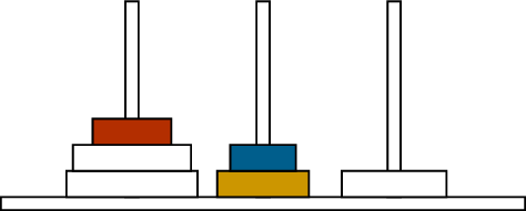
A mid-game stateThe next moveAnother move
Two moves in the Towers of Hanoi puzzle
For our first example, let’s return to the Towers of Hanoi puzzle,
discussed in Chapter 1 and illustrated in
Figure B.1. There are three
pegs and some number of disks of different sizes stacked on the pegs. In
a single move, the top disk on a peg can be moved to the top of a
different peg.
The disks stacked on a peg must always form a pyramid, with their
sizes increasing from top to bottom. This means that the smallest disk
(the one moved from Figure B.1(a) to
Figure B.1(b)) can always be moved anywhere,
but the larger disks are restricted further. From Figure B.1(b) to Figure B.1(c), we move a disk from the
middle peg to the right peg; it cannot be moved to the lft peg instead,
because then it would be on top of a smaller disk.
Initially, the disks are all placed on one peg (forming a pyramid, as
they always must). The goal of the puzzle is to move all the disks from
one peg to another. Our first task in this chapter will be to prove that
this puzzle always has a solution.
Theorem B.1. No matter how many disks there are,
it is possible to solve the Towers of Hanoi puzzle, starting with all
the disks stacked in a pyramid on any peg, and ending with all the disks
stacked in a pyramid on any other peg.
If you try to solve this puzzle by moving disks at random, you will
not get very far. (I can confirm this experimentally. For the six-disk
puzzle in Figure B.1, I performed
\(1000\) computer-simulated attempts to
solve the puzzle by randomly chosen valid moves. The median number of
moves required to move all six disks onto a peg other than the starting
one was \(8488\).) The reason for this
is that it’s very rare to see a state where one of the larger disks can
be moved.
If the largest disk in an \(n\)-disk Towers of Hanoi puzzle can be
moved from the starting peg, how must the disks be arranged?
First of all, none of them can be on top
of the largest disk. Second, the destination peg to which we want to
move the largest disk must also be empty, because the largest disk can’t
be placed on top of any other. Therefore all \(n-1\) other disks must be stacked onto a
third peg.
In order to achieve this state, we must move the top \(n-1\) disks from one peg to another. In
this process, we can ignore the largest disk, which means that we are
effectively solving a Towers of Hanoi puzzle with one fewer disk. This
makes the problem a perfect setup for an induction proof!
Proof of Theorem B.1. We induct on \(n\), the number of disks. When \(n=1\), we can move the disk from one peg to
another in a single step. So the base case holds.
Assume that there is a way to move \(n-1\) disks from any peg to any other. Then
there is also a solution to the \(n\)-disk puzzle, from any starting peg to
any ending peg.
Using the \((n-1)\)-disk
solution, move the first \(n-1\) disks
from the starting peg to the third peg (which is neither the starting
nor the ending peg).
Move the largest disk from the starting peg to the ending
peg.
Using the \((n-1)\)-disk
solution again, move the first \(n-1\)
disks from the third peg to the ending peg.
By induction, there is a solution for all \(n\). ◻
This example demonstrates the structure of a proof by induction.
Although there are more complicated variants that bend or break some of
the rules, an ordinary proof by induction has the following
characteristics:
We must be trying to prove a statement with many cases which can
be numbered, usually starting at \(0\)
or \(1\).
The first sentence, “We induct on \(n\), the number of disks,” is a standard
way to explain what the cases are (they are the different versions of
the puzzle with different numbers of disks) and how they can be numbered
(according to the number of disks, which we are now going to refer to as
\(n\)).
We must begin with a base case: a self-contained
proof of the first case of the statement.
Here, that’s the \(n=1\) case, so at
the beginning of the proof, we explain how to solve the \(1\)-disk problem. As in this example,
usually the proof of the base case is very short.
The other part of the proof is an induction
step: a proof that if any given case of the theorem is true,
then the next case is also true.
As usual, a direct proof of an “if \(P\), then \(Q\)” statement begins by assuming \(P\), and trying to prove \(Q\). So we begin the induction step by
assuming that the theorem holds in some case, and using this assumption
to prove that the theorem also holds in the next case. We refer to this
assumption as the induction hypothesis.
The induction step can be written in several slightly different ways.
We can assume the \(n\)th
case of the theorem and prove the \((n+1)\)th, or assume the \((n-1)\)th case of the theorem
and prove the \(n\)th case.
We can introduce a new variable, proving that if the theorem holds when
\(n=k\), it also holds when \(n=k+1\) (or that if the theorem holds when
\(n=k-1\), it also holds when \(n=k\)). The choice between these is mostly
a matter of taste.
I suspect that many of my readers have already seen proofs by
induction, but I am carefully explaining it anyway, because it’s a very
tricky idea when you first learn it.
It’s also often taught without explaining how or why it works. To
give you an intuitive understanding, let’s prove a few cases of
Theorem B.1 without using induction. (In all of
these lemmas, by “the puzzle has a solution”, we mean that we can move
all the disks from any peg to any other peg.)
Lemma B.2. The Towers of Hanoi puzzle with \(1\) disk has a solution.
Proof. When no other disks interfere, we can move the disk
from any peg to any other in a single step. ◻
Lemma B.3. The Towers of Hanoi puzzle with \(2\) disks has a solution.
Proof. By Lemma B.2, there
is a way to move the smallest disk to a different peg. Using this
method, move the smallest disk from the starting peg to a third peg:
neither the starting nor the ending peg. (In this process, the largest
disk won’t get in the way, because any other disks can be placed on top
of it.)
Now the largest disk is free, and the ending peg is empty, so the
largest disk can be moved to the ending peg.
Finally, using the method of Lemma B.2 again,
we can move the smallest disk from the peg it’s on to the ending peg,
which leads to the arrangement we wanted. ◻
Lemma B.4. The Towers of Hanoi puzzle with \(3\) disks has a solution.
Proof. By Lemma B.3, there
is a way to move the \(2\) smallest
disks to a different peg. Using this method, move the \(2\) smallest disks from the starting peg to
a third peg: neither the starting nor the ending peg. (In this process,
the largest disk won’t get in the way, because any other disks can be
placed on top of it.)
Now the largest disk is free, and the ending peg is empty, so the
largest disk can be moved to the ending peg.
Finally, using the method of Lemma B.2 again,
we can move the \(2\) smallest disks
from the peg they’re on on to the ending peg, which leads to the
arrangement we wanted. ◻
Lemma B.5. The Towers of Hanoi puzzle with \(4\) disks has a solution.
Proof. By Lemma B.4, there
is a way to move the \(3\) smallest
disks to a different peg. Using this method, move the \(3\) smallest disks from the starting peg to
a third peg: neither the starting nor the ending peg. (In this process,
the largest disk won’t get in the way, because any other disks can be
placed on top of it.)
Now the largest disk is free, and the ending peg is empty, so the
largest disk can be moved to the ending peg.
Finally, using the method of Lemma B.2 again,
we can move the \(3\) smallest disks
from the peg they’re on on to the ending peg, which leads to the
arrangement we wanted. ◻
They are almost identical: they only
differ in the number used and in the lemma referenced. (In the case of
Lemma B.3, some plural nouns become
singular, but that’s just a quirk of the English language.)
It is clear that if we wanted to write a proof of a lemma for \(5\) disks, or \(6\) disks, or \(64\) disks, we could do it by copying and
pasting and then changing the numbers. So as soon as we have a template
which we can copy and paste, we should accept that all those lemmas are
true: we know how to obtain a proof of any of them.
This is the logic underlying a proof by induction. The template that
we would copy and paste is exactly the induction step, with specific
numbers replaced by \(n-1\) or \(n\).
In this copying-and-pasting view of
induction, why do we need to prove the base case?
Because the proof of Lemma B.2 didn’t follow the template: at
that point, we didn’t have a previous lemma we could cite. So the proof
by induction must tell us how to prove the first lemma, as well as how
to prove every other lemma.
A common modification to the basic induction template is
strong induction, where we allow each case of the
theorem to rely on multiple smaller cases, and not just the immediately
preceding case. For example, if the \(6\)-disk solution involved using a \(5\)-disk solution and a \(4\)-disk solution, or if it unpredictably
went back to a \(k\)-disk solution for
some unknown \(k \in \{1,2,3,4,5\}\),
then we’d have to use strong induction.
Why is this still okay?
Because there is no circular reasoning. If
we take all the cases the \(n\)th case depends on, and then
all the cases they depend on, and so on, eventually we end up going back
to the base case.
I want to devote most of this chapter to discussing the way induction
works in graph theory in particular, but first I want to give one last
general piece of advice.
A common tip for getting started solving a problem is to try small
cases of the problem first. It is easier to solve specific small
examples than to solve a general problem, and by looking at the
examples, you can try to make guesses about a general solution. What I
want to tell you about is a related idea: if you think you might want to
use induction to solve a problem, don’t look at the small cases on their
own! Look at consecutive cases together, trying to get an idea of what
your induction step might be by seeing how one small case can be used to
get the next.
So, for example, no matter how you want to solve the Towers of Hanoi
puzzle, it’s reasonable to look at what happens for \(2\) or \(3\) disks to start with. If you want to try
a proof by induction, you should look at the \(2\)-disk solution and \(3\)-disk solution side by side, and try to
draw connections between the two.
In this case, you might find the \(2\)-disk solution inside the \(3\)-disk solution: once, or even twice. You
might also arrive at a useful insight by comparing the lengths of the
solutions. Hypothetically, the relationship could have been different:
the \(3\)-disk solution could be the
\(2\)-disk solution with a short
sequence added to the end, or inserted in the middle, or with some
transformation applied to each step.
Induction on graphs
In graph theory, induction is often used in a special way that’s
slightly different from induction in many other areas of math. Instead
of proving that a statement is true for all natural numbers \(n\), we often try to prove it for all
graphs, or at least for all graphs with some property relevant to the
specific problem.
This tends to work out reasonably well for us, because we have at
least two good ways of measuring how big a graph is: we can count the
vertices, or we can count the edges. The most common technique is to
induct on the number of vertices in a graph. Here, we consider “the
statement is true for all graphs with \(n\) vertices” to be a single case, and
advance through these cases by induction on \(n\). (I will say more later about inducting
on the number of edges later; it is less common.)
However, because we’re grouping together many graphs into one case,
we have to be very careful about how we set up the induction. If we’re
not, we can make mistakes and prove false statements, or give incorrect
proofs of true statements. The second possibility is harder to catch,
because you won’t be able to find any counterexamples. To avoid
confusing you too much, I will give you an example of the first
possibility: a claim that is definitely false.
Claim B.6 (False claim). For all \(n\ge 3\), if \(G\) is an \(n\)-vertex graph in which every vertex has
degree at least \(2\), then \(G\) must have at least \(2n-3\) edges.
We know this is false, because the cycle graph \(C_n\) is a counterexample. Every vertex of
\(C_n\) has degree \(2\), but \(C_n\) only has \(n\) edges, which is less than \(2n-3\) for large \(n\).
Incorrect proof. We induct on \(n\). When \(n=3\), the claim holds, because we need all
\(3\) edges in a \(3\)-vertex graph to exist in order for the
assumption to hold, and \(3 =
2(3)-3\).
Assume the claim holds for all \((n-1)\)-vertex graphs: if every in an \((n-1)\)-vertex graph has degree at least
\(2\), then the number of edges is at
least \(2(n-1)-3\) or \(2n-5\). To get an \(n\)-vertex graph, we add a vertex; to give
it degree at least \(2\), we need to
add at least two new edges. This results in a graph with at least \((2n-5)+2\) or at last \(2n-3\) edges.
By induction, the claim is true for all \(n\). ◻
Just knowing that this proof is incorrect is not enough. We need to
understand why it is incorrect, to make sure that we do not
do it again.
The smallest counterexample to Claim B.6 is \(C_4\). Why does the proof fail to consider
\(C_4\)?
When going from \(3\)-vertex graphs to \(4\)-vertex graphs, we try to add a vertex
of degree \(2\) to a \(3\)-vertex graph with minimum degree \(2\). But \(C_4\) cannot be obtained in this way: if
you remove a vertex from it, you’re left with \(P_3\), which is not a graph
with minimum degree \(2\).
To avoid this mistake, I have a general theory to propose, and also a
practical solution.
The general theory is this. If the possible cases of our theorem were
truly the positive integers \(n\ge 3\),
they would form a chain: \[3 \to 4 \to 5 \to
6 \to 7 \to 8 \to 9 \to 10 \to \dots\] If we start at \(3\) and follow the arrows, we will
eventually get to every possibility.
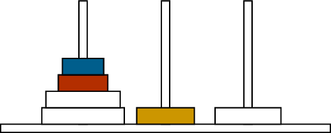
But in Claim B.6, the set of possible
cases is really the set of graphs with minimum degree at least \(2\). Instead of a chain, we can imagine
organizing this set into an infinite diagram, a fragment of which is
shown in Figure B.2. Here, the arrows represent
possible ways to go from a small graph to a bigger one by adding a new
vertex of degree \(2\).
Organizing the graphs with minimum degree at least \(2\) according to the induction step of
Claim B.6 (not all \(5\)-vertex graphs are
included)
If this is the induction step we intend to use, then a single \(3\)-vertex base case is not enough: by
following arrows from that case, we miss many possibilities. We could
conceivably write an induction in this way, but we would need many base
cases: all the graphs which are not obtained from a smaller
graph by following an arrow. At a bare minimum, this includes the cycle
graphs, but eventually there are other examples like this. I don’t think
this is a reasonable way to write an induction proof; I’m just saying
that if we wanted to rescue this idea, that’s what we’d have to do.
Is there a \(5\)-vertex graph with minimum degree at
least \(2\), other than \(C_5\), which is not obtained by adding a
vertex to a smaller graph of minimum degree at least \(2\)?
Yes: we can get another such graph by
taking two copies of \(K_3\) that share
a vertex of degree \(4\).
I did, however, promise a practical solution to the problem. This
practical solution restricts the way we can write proofs by induction on
the vertices of \(G\), allowing only
ones that are guaranteed to work. You can think of it as filling in the
blanks in the following template:
Theorem B.7 (Induction Template). If a graph
\(G\) has property \(A\), it also has property \(B\).
Proof. We induct on the number of vertices in \(G\). (Prove a base case
here.)
Now, for some \(n>1\)(or
other lower bound, depending on the base case), assume that all
\((n-1)\)-vertex graphs with property
\(A\) also have property \(B\). Let \(G\) be an \(n\)-vertex graph with property \(A\). Our goal is to show that \(G\) also has property \(B\).
Let \(x\) be a vertex of \(G\)(usually chosen by some clever
rule you’ll have to come up with). Then \(G-x\) (the graph obtained from \(G\) by deleting \(x\) and all edges out of \(x\)) also has property \(A\)(by an argument related to the
way we chose which vertex to delete).
By the induction hypothesis, \(G-x\)
also has property \(B\). When we add
back the vertex \(x\), \(G\) also has property \(B\)(by another argument you’ll
have to come up with).
By induction, all graphs with property \(A\) also have property \(B\). ◻
Why does this work, when our previous argument didn’t? The key is the
step “Let \(G\) be an \(n\)-vertex graph with property \(A\).” We didn’t make any assumptions about
\(G\). Rather, we started from an
arbitrary graph with property \(A\); to
apply the induction hypothesis, we cooked up a graph \(G-x\) which is an \((n-1)\)-vertex graph with property \(A\).
Another way to put it is this: using this induction template prevents
the induction from having the kind of structure shown in Figure B.2, by forcing each graph
\(G\) to have a previous case \(G-x\) it is obtained from. Only the graphs
covered in the base case are exempt from this.
Using the induction template takes practice to master. (A good
example of its use early on in this book is in the proof of Lemma 4.6.) However, it
is also helpful, because it is a scaffolding for your proofs by
induction: it means you don’t have to start from scratch.
Earlier, I mentioned induction on the number of edges of a graph.
This is only done a few times in this book:
When proving the handshake lemma (Lemma 4.1) and later when
proving its directed version, Lemma 7.1.
When proving Theorem 10.1 on the number of connected
components in a graph with \(m\)
edges.
When proving Euler’s formula (Theorem 21.4) for plane
embeddings.
We can use a variant of the induction template here, deleting an edge
\(xy\) rather than a vertex \(x\). (The proof of Theorem 8.3 uses strong induction: we
delete multiple edges at once.) Repeatedly deleting edges leaves a graph
with no edges, but the same number of vertices; all such graphs should
be our base cases.
Inductive definitions
Some structures in graph theory are important because they make it
particularly easy to write a proof by induction. There are two that I
can point to in this book:
Trees, which are introduced in Chapter 9. Lemma 10.6 tells us that if \(T\) is a tree and \(x\) is a degree-\(1\) vertex, then \(T-x\) is a tree; moreover, we know from
Lemma 10.5 that every tree with
multiple vertices has some degree-\(1\)
vertices to use Lemma 10.6 with.
Used in reverse, these two lemmas give us an “inductive definition”
of a tree: a tree is either a graph with \(1\) vertex, or a graph obtained from a
smaller tree by adding a new vertex of degree \(1\).
\(2\)-connected graphs, which
are introduced in Chapter 25. Theorem 25.4 tells
us that every \(2\)-connected graph has
an ear decomposition, which gives us an inductive definition of a \(2\)-connected graph: it is either a cycle,
or a graph obtained from a smaller \(2\)-connected graph by adding an
ear.
I don’t want to spoil the details of these objects if you haven’t
read those chapters, even if you’re dying to know what it means to add
an ear to a graph. But what do I mean by an inductive definition?
Well, in both cases, we are saying something like, “A (type of graph)
is either a (base case) or obtained from a smaller (same type of graph)
by adding a (small modification).” This is what I mean by an
inductive definition. You can see how it resembles the
structure of a proof by induction—it also makes it easy to write
one.
How can we write a proof by induction
using an inductive definition?
The base case of the induction is to
check that our theorem is true in the base case of the definition.
The induction step is to check that if the theorem is true for a
graph of this type, it remains true after the small
modification.
I want to show you how inductive definitions work in graph theory
without getting into either of the advanced examples we learn about
elsewhere in the book. So I will give you a different example: a family
of graphs called threshold graphs. These were defined by Václav
Chvátal and Peter Hammer in 1977 to study when multiple inequalities
with \(\{0,1\}\)-valued variables can
be combined into one [18].
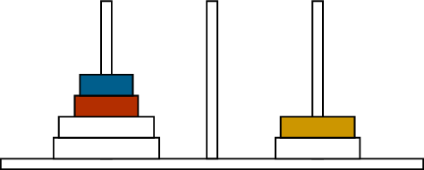
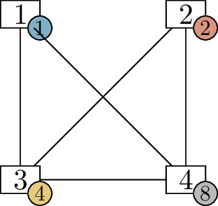
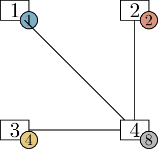
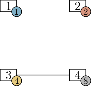
\(t=4\)\(t=8\)\(t=11\)
\(4\)-vertex threshold
graphs with three thresholds \(t\)
Threshold graphs have two definitions. One is the definition they get
their name from. A graph \(G\) is a
threshold graph if there is a function \(f
\colon V(G) \to \mathbb R\) and a value \(t \in \mathbb R\) such that two vertices
\(x\) and \(y\) are adjacent if and only if \(f(x) + f(y) > t\). In other words,
adjacency is defined by the sum of vertex labels exceeding a threshold.
Figure B.3 shows three examples of
\(4\)-vertex threshold graphs: here,
the values of \(f\) are \(0.3, 0.6, 1.2, 2.4\) in all three diagrams,
but we require different thresholds \(t\) for an edge to exist.
The other definition is the inductive definition. A graph \(G\) is a threshold graph if it has only one
vertex, or if it can be obtained from a smaller threshold graph in one
of two ways:
adding a new vertex of degree \(0\), or
adding a new vertex adjacent to all existing vertices.
Let’s practice induction by proving that we get the same class of
graphs by either definition!
After I wrote down the proof below for the first time, I realized
that I spent half a page just on writing “threshold graph by the …
definition” many times. So to abbreviate, let’s call \(G\) a thres graph if it satisfies
the inequality definition, and a hold graph if it satisfies the
inductive definition.
Proposition B.8. A graph \(G\) is a thres graph if and only if it is a
hold graph.
Proof. We will need two proofs by induction, one for each
direction of the proof.
First, let’s show that if graph \(G\) is a hold graph, we can define a
function \(f \colon V(G) \to \mathbb
R\) to make it a thres graph. For simplicity, we’ll use the
threshold \(t=0\).
Our base case here is the \(1\)-vertex graph. We can give the single
vertex any value of \(f\) we like, and
it will be a thres graph, because there isn’t a pair of vertices for
which to check it.
Suppose now that for some hold graph \(G\), we’ve defined a function \(f\) that also makes it a thres graph. We
now need to show that with either of the modifications we do, we can
extend \(f\).
Suppose we add a vertex \(x\) to
\(G\) which is not adjacent to any
vertex in \(V(G)\), getting a bigger
hold graph \(G'\).
Then to extend \(f\) to a function
\(V(G') \to \mathbb R\), we define
\[f(x) := \min\{{-1} - f(y) : y \in
V(G)\}.\] For each \(y \in
V(G)\), any value of \(f(x)\)
equal to or less than \(-1 - f(y)\) is
enough to make sure that \(f(x) + f(y) \le
-1\), preventing an edge \(xy\);
we choose \(f(x)\) to be the smallest
of these values.
Suppose we add a vertex \(x\) to
\(G\) which is adjacent to every vertex
in \(V(G)\), getting a bigger hold
graph \(G''\).
Then to extend \(f\) to a function
\(V(G'') \to \mathbb R\), we
define \[f(x) := \max\{1 - f(y) : y \in
V(G)\}.\] For each \(y \in
V(G)\), any value of \(f(x)\) at
least \(1 - f(y)\) is enough to make
sure that \(f(x) + f(y) \ge 1\),
ensuring an edge \(xy\): we choose
\(f(x)\) to be the largest of these
values.
In both cases, the larger hold graph continues to be a thres graph
with the extended \(f\). We conclude
that as we build bigger and bigger hold graphs from the \(1\)-vertex graph, they always remain thres
graphs, and therefore by induction, all hold graphs are thres
graphs.
That’s one part done. Now we show that if \(G\) is a thres graph, it is also a hold
graph. Since we’re trying to establish the inductive definition, we
won’t be able to use it as a model for induction; instead, we’ll use the
induction template.
We induct on the number of vertices in \(G\). When \(G\) is a \(1\)-vertex thres graph, it is also a hold
graph by the base case of the inductive definition.
Now, for some \(n>1\), assume
that all \((n-1)\)-vertex thres graphs
are also hold graphs. Let \(G\) be a
thres graph, defined using a function \(f
\colon V(G) \to \mathbb R\) and a threshold \(t\).
For which vertices \(x\) is \(G-x\) a thres graph?
All of them: we can just keep the same
function \(f\) (with fewer inputs) and
the same threshold \(t\).
So we won’t be deleting a vertex carefully to make sure we still have
a thres graph; we’ll be deleting a vertex carefully to make it’s easy to
check the definition of a hold graph when we put it back.
I propose two options for the deletion. Let \(x\) be the vertex of \(G\) such that \(f(x)\) is as small as possible, and let
\(y\) be the vertex of \(G\) such that \(f(y)\) is as large as possible.
If \(f(x) + f(y)
\le t\), what do we know about \(x\)?
Since not even \(f(y)\) is big enough for the sum with \(f(x)\) to exceed the threshold, we know
\(f(x)+f(z) \le t\) for all vertices
\(z\), so \(x\) has no neighbors in \(G\).
In this case, consider the thres graph \(G-x\). By the induction hypothesis, \(G-x\) is also a hold graph. But \(G\) is obtained from \(G-x\) by adding a new vertex \(x\) of degree \(0\), which means \(G\) is also a hold graph.
If \(f(x) + f(y)
> t\), what can we do instead?
Since even \(f(x) + f(y)\) is bigger than \(t\), and \(f(x)\) is the smallest value of \(f\) there is, we know \(f(z) + f(y) > t\) for all vertices \(z\). Therefore \(y\) is adjacent to all other vertices of
\(G\).
In this case, consider the thres graph \(G-y\). By the induction hypothesis, \(G-y\) is also a hold graph. But \(G\) is obtained from \(G-y\) by adding a new vertex \(y\) adjacent to all existing vertices,
which means \(G\) is also a hold
graph.
In both cases, we prove \(G\) is a
hold graph, completing the induction step. By induction, all thres
graphs are hold graphs. ◻
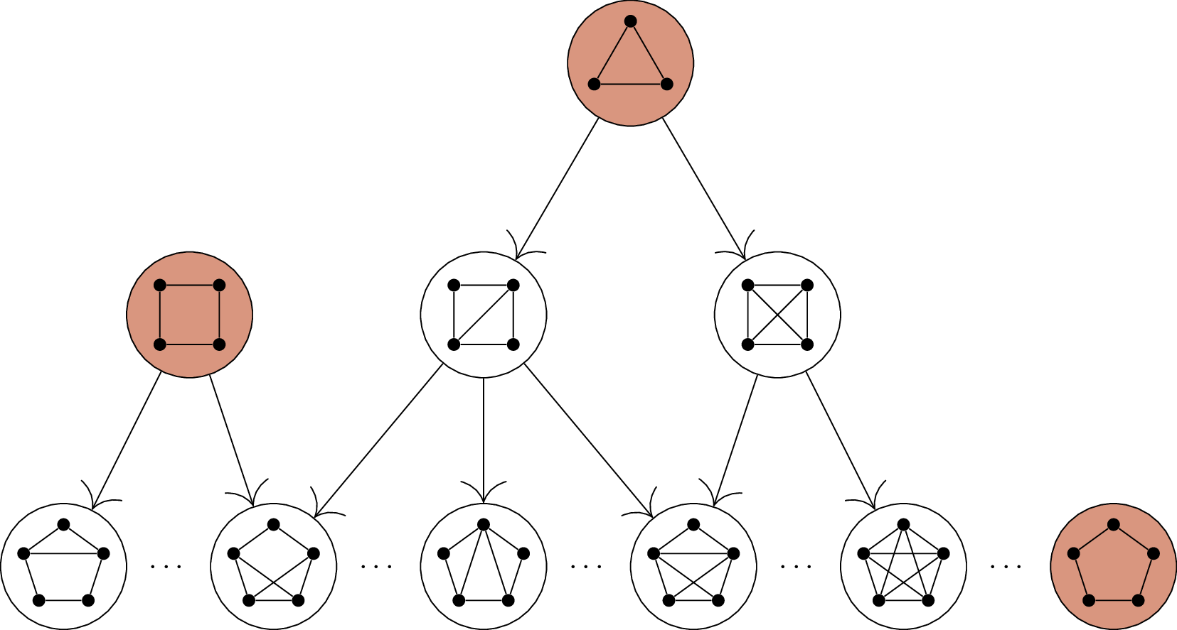
Building all threshold graphs from a \(1\)-vertex graph
We can compare the incorrect proof of the false Claim B.6 to the way that we used
an inductive definition in this proof. Actually, both proofs are written
in the same style: we start with a base case and then we grow it. The
difference is that in the case of threshold graphs, the inductive
definition guarantees that every other threshold graph can be obtained
from a \(1\)-vertex graph. (For a
demonstration of this, see Figure B.4.) In other words, one
base case is all we need!
Recursive constructions
Let’s say that a sequence of graphs \(G_1,
G_2, G_3, \dots\) has a recursive construction
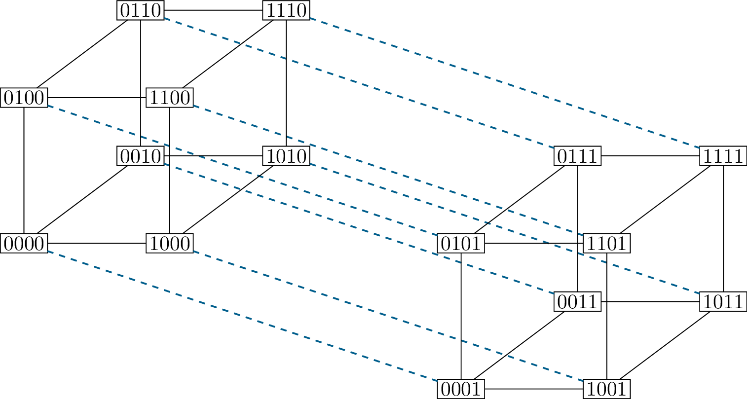
if we have a fixed procedure by which we can build \(G_n\) out of \(G_{n-1}\) for all \(n>1\). For example, the sequence \(Q_1, Q_2, Q_3,\dots\) of hypercube graphs
defined in Chapter 4 has a recursive construction.
For all \(n\), we can build \(Q_n\) from \(Q_{n-1}\) by the following procedure:
Start with two disjoint copies of \(Q_{n-1}\).
If we think of the vertices of \(Q_{n-1}\) as \((n-1)\)-bit strings, then we can say that
the first copy of \(Q_{n-1}\) has a
vertex \(x0\) (\(x\), followed by a \(0\)) for every vertex \(x \in V(Q_{n-1})\), and the second copy of
\(Q_{n-1}\) has a vertex \(x1\) for every vertex \(x \in V(Q_{n-1})\).
In addition to the edges that already exist within each copy of
\(Q_{n-1}\), add an edge \(\{x0, x1\}\) for all \(x \in V(Q_{n-1})\): this is an edge between
the two vertices corresponding to \(x\)
in the two copies of \(Q_{n-1}\).
This is easier to see in a diagram. Figure B.5 shows how we build
\(Q_4\) using this recursive
construction: the two copies of \(Q_3\)
are shown on the left (with a \(0\) at
the end of every vertex) and on the right (with a \(1\) at the end of every vertex), and the
dashed edges are the edges added between the copies.
Using a recursive construction to build \(Q_4\) from two copies of \(Q_3\)
Other notable examples of recursive constructions in this book
include:
The Mycielski graphs defined in Chapter 19: each graph is the
Mycielskian of the previous graph.
The de Bruijn digraphs defined in Chapter 20: by
Proposition 20.3, for all
\(k\ge 1\), each digraph in the
sequence \(B(k,1), B(k,2), B(k,3),
\dots\) is the line digraph of the previous graph.
The iterated barycentric subdivisions used as an example in
Chapter 21: to go from each plane
embedding to the next, take the barycentric subdivision of every
triangular face.
In general, the word “iterated” in a mathematical term often
indicates a recursive construction.
Why do I mention recursive constructions here? You can probably guess
why: induction is a good way to prove properties of a sequence of graphs
with a recursive construction.
Let’s start with a simple example, where the proof by induction is
actually much more complicated than what we need.
Proposition B.9. For all \(n\ge 1\), the hypercube graph \(Q_n\) has \(2^n\) vertices and \(n \cdot 2^{n-1}\) edges.
Proof. We induct on \(n\).
When \(n=1\), the hypercube graph \(Q_1\) has two vertices (\(0\) and \(1\)) and one edge between them. Since \(2^1 = 1\) and \(1
\cdot 2^{1-1} = 1\), both formulas we want to prove are true for
\(n=1\).
Now assume, for some \(n>1\),
that \(Q_{n-1}\) has \(2^{n-1}\) vertices and \((n-1) \cdot 2^{n-2}\) edges. When we
construct \(Q_n\) recursively, we take
two disjoint copies of \(Q_{n-1}\), so
we get \(2 \cdot 2^{n-1}\) or \(2^n\) vertices. There are \((n-1) \cdot 2^{n-2}\) edges in each copy of
\(Q_{n-1}\), and \(2^{n-1}\) edges added between them (one for
each vertex of \(Q_{n-1}\)), for a
total of \[(n-1) \cdot 2^{n-2} + (n-1) \cdot
2^{n-2} + 2^{n-1} = n \cdot 2^{n-1}\] edges.1
We confirm that if \(Q_{n-1}\) has
the number of vertices and edges we wanted, then so does \(Q_n\). By induction, the formulas in the
proposition hold for all \(n\ge
1\). ◻
What’s the much simpler way to prove that
\(Q_n\) has \(n\cdot 2^{n-1}\) edges?
Use the handshake lemma! There are \(2^n\) vertices, and each vertex has degree
\(n\), so the sum of degrees is \(n \cdot 2^n\), and to get the number of
edges, we divide by \(2\).
If we didn’t know the formula \(n\cdot 2^{n-1}\) ahead of time, could we
still use a proof by induction?
Yes, but we’d have to solve a recurrence
relation to figure out the formula, first. If \(f(n)\) is the number of edges, then the
argument in our induction step tells us that \(f(n) = 2 \cdot f(n-1) + 2^{n-1}\), with
\(f(1)=1\).
Here’s a quick algebraic way to solve the recurrence relation: first,
divide through by \(2^n\) to get \(\frac{f(n)}{2^n} = \frac{f(n-1)}{2^{n-1}} +
\frac12\). Now, each occurrence of \(f(k)\) for any \(k\) shows up divided by \(2^k\), so we can define \(g(n) = \frac{f(n)}{2^n}\). This has the
initial value \(g(1) = \frac{f(1)}{2} =
\frac12\) and a much simpler recurrence relation: \(g(n) = g(n-1) + \frac12\). If we start with
\(\frac12\) and add \(\frac12\) each time, then we should get
\(g(n) = \frac n2\), and so \(f(n) = g(n) \cdot 2^n = n \cdot
2^{n-1}\).
This trick can be used to solve many recurrence relations, but first
you have to figure out the right thing to multiply or divide by in order
to simplify the recurrence relation.
Here is a second example of induction on \(Q_n\), for which we’ll have to work
harder.
Proposition B.10. For all \(n \ge 1\), the diameter of \(Q_n\) (the largest distance between any two
of its vertices) is \(n\).
Proof. When \(n=1\), \(Q_n\) is still the graph with two vertices
and \(1\) edge; this has diameter \(1\), because the two vertices are at
distance \(1\) from each other.
Now assume, for some \(n>1\),
that \(Q_{n-1}\) has diameter \(n-1\); to prove the induction step, we
would like to prove that \(Q_n\) has
diameter \(n\).
On the level of walks in a graph, what
does our induction hypothesis tell us, and what do we need to
prove?
We know that for every pair \(x,y\) of vertices in \(Q_{n-1}\), there is an \(x-y\) walk of length at most \(n-1\), and that there is some pair \(x,y\) for which no shorter walk exists.
We want to show that for every pair \(x,y\) of vertices in \(Q_n\), there is an \(x-y\) walk of length at most \(n\), and we want to find some pair \(x,y\) for which we prove that no shorter
walk exists.
First, let’s prove that walks of length at most \(n\) exist between every pair of vertices in
\(Q_n\). If we take two vertices in the
same copy of \(Q_{n-1}\), then there is
a walk of length at most \(n-1\)
between them, by the induction hypothesis. So suppose we take two
vertices in different copies: without loss of generality, vertices of
the form \(x0\) and \(y1\).
By the induction hypothesis, there is an \(x-y\) walk in \(Q_{n-1}\) of length at most \(n-1\); equivalently, an \(x0 - y0\) walk in the first copy of \(Q_{n-1}\) inside \(Q_n\). By taking that \(x0 - y0\) walk, and adding the vertex \(y1\) to the end (which is adjacent to \(y0\)), we get an \(x0 - y1\) walk whose length is only
increased by \(1\): the length is most
\(n\), as we wanted.
To find a pair of vertices at distance \(n\), we begin with other half of our
induction hypothesis: that \(Q_{n-1}\)
contains two vertices \(x,y\) for which
all \(x-y\) walks have length at least
\(n-1\).
Using \(x\) and \(y\), which vertices in \(Q_n\) should we pick that we expect to be
at distance \(n\)?
Vertices \(x0\) and \(y1\), for example: these are as far away as
possible and also in different copies of \(Q_{n-1}\).
We can think of a walk in \(Q_n\) is
a sequence of steps where at each step, we change some coordinate. To
get from \(x0\) to \(y1\), at least once, we need to change the
last coordinate, going from \(z0\) to
\(z1\) for some \(z\). Let’s just skip all steps where we do
that: we will now get a walk from \(x0\) to \(y0\) in the first copy of \(Q_{n-1}\), and it will be shorter by at
least one step.
What is the motivation for doing
this?
Our induction hypothesis is an assumption
about all \(x-y\) walks, so in order to
use it, we first need to obtain an \(x-y\) walk to apply it to!
This new \(x0 - y0\) walk
corresponds to an \(x-y\) walk in \(Q_{n-1}\), so it has length at least \(n-1\), by our induction hypothesis. The
\(x0 - y1\) walk has at least one step
we skipped, so it has length at least \(n\), completing our lengthy induction
step.
We’ve proved that if \(Q_{n-1}\) has
diameter \(n-1\), then \(Q_n\) has diameter \(n\); by induction, \(Q_n\) has diameter \(n\) for all \(n\ge 1\). ◻
For \(n=3\) disks, write down
the steps of the solution that the proof gives us.
In general, in terms of \(n\),
how many steps are there in the solution?
It turns out that the number in part (b) is the least number of
steps required to move all the disks from one peg to another. Prove this
claim by induction.
The sequence \(F_0, F_1, F_2,
\dots\) of Fibonacci numbers is defined by \(F_0 = 0\), \(F_1
= 1\), and the recurrence relation \(F_n = F_{n-1} + F_{n-2}\) for all \(n\ge 2\).
A matching is defined in Chapter 13
as a spanning subgraph \(M\) where
every vertex has degree \(0\) or \(1\); equivalently, the edges \(E(M)\) share no endpoints.
Prove that for all \(n\ge 1\),
the path graph \(P_n\) has \(F_{n+1}\) matchings.
Prove that for all \(n\ge 3\),
the cycle graph \(C_n\) has \(F_{n+1} + F_{n-1}\) matchings.
Prove by induction on \(n\) that
for all \(n\ge 5\), there exists a
graph with \(n\) vertices and \(2n-4\) edges which has minimum degree \(2\) and maximum degree \(4\).
Prove that the complement of every threshold graph is also a
threshold graph.
Let’s say that a graph \(G\) has
“comparable neighborhoods” if, for all \(x,y
\in V(G)\), either vertex \(x\)
is adjacent to all the neighbors of \(y\), or vertex \(y\) is adjacent to all the neighbors of
\(x\). (That is, the
neighborhoods\(N(\{x\})\) and
\(N(\{y\})\) are comparable
sets, following definitions in Chapter 15.)
Prove that every threshold graph has comparable
neighborhoods.
In the bottom level of Figure B.4, \(8\) of the \(11\) possible four-vertex graphs are shown
(up to isomorphism). The missing \(3\)
graphs are exactly the \(3\) graphs
that do not have comparable neighborhoods. What are they?
Let \(G\) be a graph with
comparable neighborhoods. Prove that it either has a vertex adjacent to
every other vertex, or a vertex with no neighbors.
Prove by induction that if \(G\)
has comparable neighborhoods, it is a threshold graph.
Let a “quadsum graph” be a graph on at least \(4\) vertices which is either a \(4\)-vertex cycle or a union \(G \cup H\) where \(G\) and \(H\) are quadsum graphs with \(2\) vertices and \(0\) edges in common.
Prove that all \(n\)-vertex quadsum
graphs have the same number of edges, and find that number as a function
of \(n\).
Let a “Hanoi integer” be an integer in which no two adjacent
digits are equal (such as 123456, or 271828, but not 144702). We define
two operations on Hanoi integers:
A “tweak” changes the last digit to anything else that’s not the same
as the previous digit: for example, we may change 123456 to 123450.
A “twiddle” takes the longest suffix of two digits alternating, as
\(\dots xyxy\), and switches the two
digits: we may change 123456 to 123465, or 271828 to 271282, or 363636
to 636363. Twiddles are forbidden if they would put a 0 at the beginning
of the integer.
Prove that you can change any \(n\)-digit Hanoi integer to any other with a
combination of \(2^n - 1\) tweaks and
twiddles.
Prove that \(2^n-1\) operations
are required to get from a number written only with the digits 0–4 to a
number written only with the digits 5–9.
Footnotes
It can be tempting to slack off when verifying this
identity, since we know what we should get when we simplify
if the proof by induction is going to work. Try to resist this
temptation and actually do the algebra, or else you risk proving
something false one day.↩︎