Without learning about walks in a graph first, we would find it hard
to study almost anything else. Do you want to understand regular graphs
(Chapter 5)? Cycles are the
quintessential regular graph. Euler tours (Chapter 8)? A
kind of closed walk. Trees (Chapter 9)? They are
connected, and they have no cycles, both properties that come back to
this chapter. Matchings (Chapter 13)? Understanding
augmenting paths is key to finding larger matchings. I could go on, but
I already have a section devoted to topics that this chapter will help
you understand: the table of contents.
This chapter is one of the first in which different will give you
slightly different definitions of the concepts we introduce. I have
chosen to define paths and cycles as subgraphs which are represented by,
but not the same as, walks. Other authors say that paths and cycles are
a type of walk, and still other authors use the word “path” to mean
“walk” and say “simple path” instead of “path”. In my opinion, the
terminology I’ve picked is the terminology that best reflects actual
usage by mathematicians: no matter how we define paths and cycles, we
treat them as subgraphs, count them as subgraphs, and do things with
them that can only be done with graphs. By saying that a walk
represents a path or cycle, I also help us remember that there
can be multiple such representations.
Anyway, justification aside, this also goes to warn you that in graph
theory, not every source you read will give you the same definitions.
The definitions should be interchangeable, once you learn how. After
all, all graph theorists are still doing the same math, no matter how we
talk about it.
I include the proof of Theorem 3.1 in
this chapter, because it would be strange to postpone the proof to an
appendix; however, the natural place to study the proof is in
Appendix A, because it is
a good early example of a proof by the extremal principle. Similarly,
Lemma 3.3 is a good example of unpacking
definitions, which I also discuss in Appendix A.
Walks and paths
Last time we looked at walks in a graph, it was in the context of the
Towers of Hanoi puzzle, in Chapter 1; this time, let’s look at
a simpler puzzle.
The state graph of the three cup puzzleNot a solution
The three cup puzzle
To set up this puzzle, you will need three empty cups; ideally, they
are empty mugs of beer, because this puzzle is not difficult enough to
challenge anyone sober for very long. They are placed in a row on the
table, right side up: \(\sqcup\sqcup\sqcup\). A valid move in this
puzzle is to take two cups that are next to each other—the first two, or
the last two—and flip them over. From the starting state, a single move
can take us to the \(\sqcap\sqcap\sqcup\) state if the first two
cups are flipped, or to the \(\sqcup\sqcap\sqcap\) state if the last two
cups are flipped. The goal of the puzzle is to flip all three cups
upside down.1
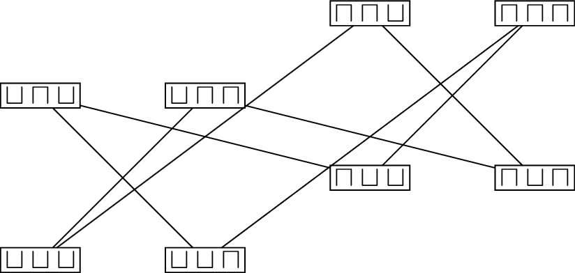
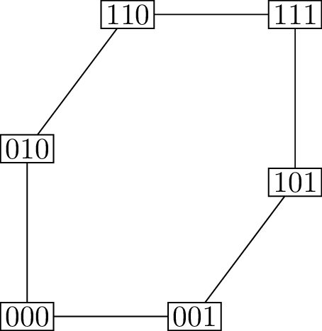
Figure 3.1(a) shows a graph of all the
states possible in the three cup puzzle, where two vertices are adjacent
if it’s possible to move from one state to the other. (This is a
symmetric relation, because all valid moves are reversible.)
In Chapter 2, we defined paths
in a graph \(G\): copies of the path
graph \(P_n\), for some \(n\). A big part of the reason why we define
paths is exactly to describe situations like the three cup puzzle. For
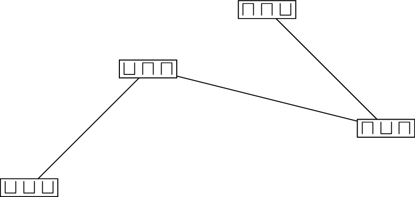
example, the subgraph shown in Figure 3.1(b)
is a \(4\)-vertex path. By following
the edges of the path, we can get from \(\sqcup\sqcup\sqcup\) to \(\sqcap\sqcap\sqcup\). If only we could find
a different subgraph: a path which included vertices \(\sqcap\sqcup\sqcap\) and \(\sqcap\sqcap\sqcap\). This would tell us
how to solve the impossible puzzle!
It’s frequently useful to summarize a path by listing all the
vertices along it from one end to the other; for example, for the path
in Figure 3.1(b), we could write down the
sequence \[(\sqcup\sqcup\sqcup, \;
\sqcup\sqcap\sqcap, \; \sqcap\sqcup\sqcap, \;
\sqcap\sqcap\sqcup).\] In general, for a subgraph \(P\) isomorphic to \(P_n\) by the isomorphism \(\varphi \colon V(P_n) \to V(P)\), we could
write the sequence \((\varphi(1), \varphi(2),
\dots, \varphi(n))\). In such a sequence, there is an edge
between each pair of consecutive vertices.
There are other such sequences, that do not represent paths, and if
you find a suitable victim for the three cups puzzle, you will discover
many of them by writing down your victim’s fruitless attempts. For
example, the sequence \[({\sqcup\sqcup\sqcup},\;
{\sqcup\sqcap\sqcap},\;
{\sqcap\sqcup\sqcap},\;
{\sqcap\sqcap\sqcup},\;
{\sqcap\sqcup\sqcap})\] also has the property that there is an
edge between each pair of consecutive vertices, but it does not
represent a path.
Why doesn’t it represent a path?
In a sequence of the form \((\varphi(1), \varphi(2), \dots,
\varphi(n))\), all \(n\)
vertices would be different, because \(\varphi\) is an isomorphism and therefore a
bijection. Here, some vertices do repeat.
Let’s make some definitions to generalize this idea:
Definition 3.1. A walk in a
graph \(G\) is a sequence \((x_0, x_1, \dots, x_l)\) of vertices of
\(G\), such that for each \(i=1, \dots, l\), vertices \(x_{i-1}\) and \(x_i\) are adjacent: \(x_{i-1}x_i \in E(G)\). A walk whose first
vertex is \(x\) and whose last vertex
is \(y\) is an \(x-y\) walk.
A walk \((x_0, x_1, \dots,
x_l)\)represents a path \(P\) in \(G\) when \(V(P) =
\{x_0, x_1, \dots, x_l\}\) and \(E(P) =
\{x_0 x_1, x_1x_2, \dots, x_{l-1}x_l\}\); a walk represents a
path if and only if all its vertices are distinct. We say that \(P\) is an \(x-y\) path if it can be
represented by an \(x-y\)
walk.
Occasionally, such as when we discuss Euler tours in Chapter 8 or increasing walks in
Chapter 16, we will be interested in walks
for their own sake. For the most part, though, walks are convenient
because they’re an easy-to-check version of paths. To know that a
sequence of vertices is a walk, we only have to check that consecutive
vertices are adjacent. To know that a sequence of vertices represents a
path, we have to check a global condition: that none of the vertices in
the sequence repeat.
“But wait,” you might ask, “Why are you acting like we can choose
which definition to check? Surely if a problem calls for a path, we need
to find a path, and if a problem calls for a walk, we need to find a
walk.”
Well, if all we care about is whether one of these objects exists, it
turns out that it doesn’t matter which one we use! We will prove the
following theorem later in this chapter:
Theorem 3.1. Let \(x\) and \(y\) be two vertices of a graph \(G\). Then there is an \(x-y\) walk in \(G\) if and only if there is an \(x-y\) path in \(G\).
Theorem 3.1 means that if we need to prove
that one of these objects exists, it’s enough to aim for an \(x-y\) walk: this will be easier. On the
other hand, if one of our assumptions is that one of these objects
exists, we can pick either an \(x-y\)
walk or an \(x-y\) path, whichever is
convenient.
Connected graphs
Whether it’s in the three cups puzzle, the Towers of Hanoi puzzle, or
a complicated graph that appears in serious and dignified study of math,
the first question we want an answer for is the existence question:
given vertices \(x\) and \(y\), does an \(x-y\) walk exist in the graph?
In the simplest scenario, the answer is always “yes”:
Definition 3.2. A graph \(G\) is connected when an
\(x-y\) walk exists for all \(x,y \in V(G)\).
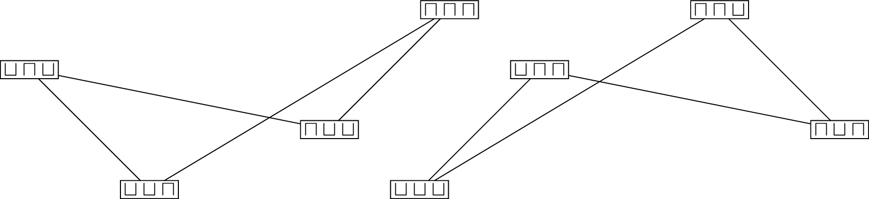
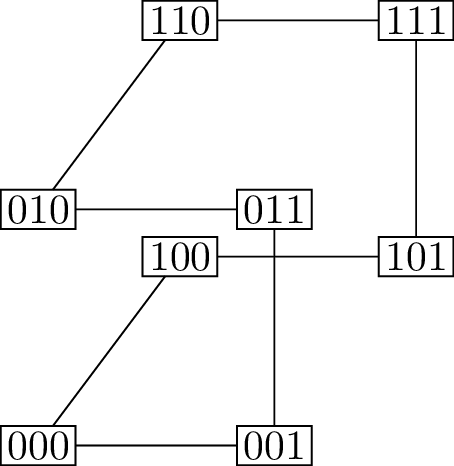
The state graph of the three cups puzzle is not connected. We can
demonstrate this fact (both in this specific example, and in general) by
showing how to split the vertex set into two parts with no edges between
them. This is done in Figure 3.2, where the two halves
are “pulled apart”: it is much easier to see here that there are no
edges between \(\{{\sqcup\sqcap\sqcup},
{\sqcup\sqcup\sqcap}, {\sqcap\sqcup\sqcup},
{\sqcap\sqcap\sqcap}\}\) and \(\{{\sqcup\sqcup\sqcup}, {\sqcup\sqcap\sqcap},
{\sqcap\sqcap\sqcup}, {\sqcap\sqcup\sqcap}\}\).
The two connected components of the three cup puzzle
graph
When a graph is defined by a sufficiently nice combinatorial rule,
such a split often comes with a reason behind it. That is the case with
the three cups puzzle. We could in theory confirm that it has no
solution by checking each of the states \(\sqcup\sqcup\sqcup\), \(\sqcup\sqcap\sqcap\), \(\sqcap\sqcap\sqcup\), and \(\sqcap\sqcup\sqcap\) to verify that all
possible moves from these states lead to another one of these states.
But we obtain the most insight—and have to exert the least effort—if we
notice that the two halves of the graph are characterized by whether the
number of \(\sqcup\)’s (cups which are
right side up) is even or odd. A move either increases the number of
\(\sqcup\)’s by two, leaves it the
same, or decreases it by two; therefore it’s impossible to go from an
odd-\(\sqcup\) state like \(\sqcup\sqcup\sqcup\) to an even-\(\sqcup\) state like \(\sqcap\sqcap\sqcap\).
Let me describe this splitting tactic more generally, by a lemma we
will be able to use in later chapters.
Lemma 3.2. For a graph \(G\), if there is a set of vertices \(S\) such that \(S\) is not empty, \(S\) is not all of \(V(G)\), and there are no edges with exactly
one endpoint in \(S\), then \(G\) is not connected.
Proof. Suppose such a set \(S\) exists; let \(x \in S\) (guaranteed to exist since \(S\) is not empty) and let \(y \in V(G) - S\) (guaranteed to exist since
\(S\) is not all of \(V(G)\)). Then we will show that there is no
\(x-y\) walk in \(G\).
Assume for contradiction that an \(x-y\) walk \((x_0, x_1, \dots, x_l)\) exists, and let
\(x_i\) be the first vertex of the walk
which is not in \(S\). Then the edge
\(x_{i-1}x_i\) has exactly one endpoint
in \(S\), contradicting our choice of
\(S\): \(x_i
\in S\), but \(x_{i-1} \notin
S\).
Why does \(x_i\) exist?
Because \(y
\notin S\), so not every vertex of the walk is in \(S\); of the vertices not in \(S\), there must be a first vertex.
Why does \(x_{i-1}\) exist? (And why should we ask
that question?)
We must ask that question because if \(i=0\), then there is no vertex “\(x_{-1}\)” in the walk. This is something we
must always watch out for when dealing with subscripts like \(i-1\) or \(i+1\). But in this case, we know \(i\ne 0\), because \(x_0 = x\) and \(x\in S\), but \(x_i \notin S\).
We’ve arrived at a contradiction, so our assumption of an \(x-y\) walk must be invalid. Therefore \(G\) is not connected. ◻
Lemma 3.2 is not a very deep result. I
want to stop and point it out anyway, because it’s important from a
proof-writing point of view. You see, when working directly from the
definition, “\(G\) is not connected” is
an awkward statement to prove: we’re trying to prove that for some
vertices \(x\) and \(y\), an \(x-y\) walk does not exist, and proving that
something does not exist is tricky. The lemma gives us a different
target to aim for: to prove that \(G\)
is not connected, we have to find the set \(S\). Moreover, the properties of \(S\) we have to check to apply the lemma are
simple ones.
A single set \(S\) is enough to show
that a graph is not connected, but sometimes it is possible to split the
graph into even more pieces with no edges between them. The most
fine-grained split possible is a split into connected components:
writing the graph \(G\) as a disjoint
union of any number of connected graphs.
Definition 3.3. The connected
components\(G_1, G_2, \dots,
G_k\) are subgraphs of \(G\)
such that
For all \(i\), \(G_i\) is connected. In other words, for all
\(x \in V(G_i)\) and \(y \in V(G_i)\), there is an \(x-y\) walk in \(G_i\) (and therefore in \(G\)).
For all \(x \in V(G_i)\) and
\(y \in V(G_j)\) where \(i\ne j\), there is no \(x-y\) walk in \(G\).
\(G\) is the disjoint union
of its connected components.
In order to satisfy the third part of the definition, connected
components must be induced subgraphs. We could define a connected
component on its own as a subgraph that is connected, but cannot be made
any bigger and still remain connected. I did not do this because I think
a big part of the definition is that together, the connected components
of \(G\) tell the entire story of when
\(x-y\) walks exist in \(G\).
Definition 3.3 is a definition that should be
accompanied by a theorem: I’ve given you no proof of the claim that
every graph can be written as the disjoint union of such subgraphs. It
is too easy to believe that this is true with no justification, so
before we prove it, let me try to persuade you that it isn’t quite so
obvious after all.
Suppose, for example, that the edges in our graphs stopped being
symmetric: that you could walk somewhere, and not be able to get back.
In that case, instead of being able to split the graph into connected
components, we’d end up with a hierarchy of vertices from which we can
reach fewer and fewer destinations—maybe even with some “dead end”
vertices that we can walk to, but never leave.
Or suppose that, unlike the infinitely-patient walker that we
imagined when defining walks, we consider a walker that gets tired, so
that our walks should contain at most (say) \(10\) steps. Then it’s possible that by
going in different directions from vertex \(x\), you can reach both vertices \(y\) and \(z\), and yet there is no component
containing \(x\), \(y\), and \(z\)—because \(y\) is too far from \(z\) to walk between the two.
So you should take a moment to appreciate the simplicity of the
answer we’re about to get to the question, “When is there an \(x-y\) walk in graph \(G\)?” It should be a bit remarkable that
the answer will be, “We can split up \(G\) into several parts called connected
components, and the answer is ‘yes’ whenever \(x\) and \(y\) are in the same part, and ‘no’
otherwise.” In a slightly different world, the answer could have been
much more complicated!
Equivalence relations
To understand the connected components of a graph \(G\), we first define a relation \(\leftrightsquigarrow\) on pairs of vertices
\(x,y \in V(G)\): \(x \leftrightsquigarrow y\) if there is an
\(x-y\) walk in \(G\). This relation is often not given any
kind of formal name, but it’s sometimes called “reachability”: \(x \leftrightsquigarrow y\) means that from
\(x\), we can reach \(y\) by following edges in \(G\).
In the three cup puzzle, for which
vertices \(x\) does \(x
\leftrightsquigarrow{\sqcup\sqcup\sqcap}\) hold?
For the vertex \(\sqcup\sqcup\sqcap\) itself, for its
neighbors \(\sqcup\sqcap\sqcup\) and
\(\sqcap\sqcap\sqcap\), and finally for
the vertex \(\sqcap\sqcup\sqcup\) that
can reach \(\sqcup\sqcup\sqcap\) in two
steps.
To proceed, we will need to prove the following result:
Lemma 3.3. The relation \(\leftrightsquigarrow\) is an equivalence
relation on \(V(G)\).
Before we do that, though, let’s talk about equivalence
relations.
You may have already seen the definition elsewhere (or not). An
equivalence relation\(\sim\)
on a set \(S\) is a relation (that is,
the statement \(x \sim y\) is either
true or false for all \(x \in S\) and
\(y \in S\)) satisfying three
poperties:
It is reflexive: for all \(x
\in S\), \(x \sim x\).
It is symmetric: for all \(x,
y\in S\), if \(x \sim y\), then
\(y \sim x\).
It is transitive: for all \(x,
y, z \in S\), if \(x\sim y\) and
\(y \sim z\), then \(x \sim z\).
But these are not just nice properties we want to prove because we
like how they sound! There is a purpose to showing that something is an
equivalence relation. These three properties are exactly the things we
need to check in order to know that we can partition \(S\) into equivalence classes: non-empty,
disjoint sets \(S_1, \dots S_k\) such
that \(S = S_1 \cup \dots \cup S_k\)
and we have \(x \sim y\) exactly when
\(x\) and \(y\) are in the same class.
In the case of our relation \(\leftrightsquigarrow\), we will use these
equivalence classes to find the connected components of \(G\).
Proof of Lemma 3.3.
Let’s check all three properties of an equivalence relation.
We check that \(\leftrightsquigarrow\) is reflexive: for
any vertex \(x\), there is an \(x-x\) walk in \(G\). Well, one such walk that’s guaranteed
to exist is the walk which is a sequence with only one term; \((x)\). There may or may not be others.
We check that \(\leftrightsquigarrow\) is symmetric: if
there is an \(x-y\) walk in \(G\), there is also a \(y-x\) walk. Well, suppose that \((u_0, u_1, \dots, u_l)\) is an \(x-y\) walk (with \(u_0 = x\) and \(u_k = y\)). Then reverse it: \((u_l, u_{l-1}, \dots, u_0)\) is a \(y-x\) walk. It starts at \(y\), ends at \(x\), and consecutive vertices in the
sequence are adjacent, because they were also consecutive in the \(y-x\) walk.
Finally, we check that \(\leftrightsquigarrow\) is transitive.
Suppose \(x,y,z\) are vertices in \(G\) such that there is an \(x-y\) walk \((u_0, u_1, \dots, u_l)\) and a \(y-z\) walk \((v_0, v_1, \dots, v_m)\). We know that
\(x = u_0\), \(y = u_l = v_0\), and \(z = v_m\). Then there is also an \(x-z\) walk: the sequence \[(u_0, u_1, \dots, u_l, v_1, v_2, \dots,
v_m).\] This definitely starts at \(x =
u_0\) and ends at \(z = v_m\).
All consecutive vertices are adjacent, because they were already
consecutive in the two walks we started with, with the exception of one
pair we need to look at more closely: \(u_l\) and \(v_1\). These are adjacent because \(u_l = y = v_0\), and \(v_0\) and \(v_1\) are consecutive in the \(y-z\) walk.
Having checked all three properties, we know that \(\leftrightsquigarrow\) is an equivalence
relation. ◻
The proof of Lemma 3.3 gives
us a useful operation on walks: we can join an \(x-y\) walk and a \(y-z\) walk to get an \(x-z\) walk.2 We
will make use of this frequently: apart from specifying a walk directly
by listing the sequence of vertices, the most common way to construct a
walk is by building it out of smaller walks.
Using Lemma 3.3 and the properties of
equivalence relations, we know that we can partition \(V(G)\) into equivalence classes of \(\leftrightsquigarrow\). These equivalence
classes are non-empty sets \(V_1, V_2, \dots,
V_k\) satisfying three properties:
They are pairwise disjoint: if \(i \ne
j\), then \(V_i \cap V_j =
\varnothing\).
Together, they include all the vertices: \(V_1 \cup V_2 \cup \dots \cup V_k =
V(G)\).
For \(x,y \in V(G)\), we have
\(x \leftrightsquigarrow y\) if and
only if there is a single \(V_i\) such
that \(x \in V_i\) and \(y \in V_i\).
These three properties are exactly what we need to say what the
connected components of \(G\) are, and
prove the following theorem:
Theorem 3.4. Any graph \(G\) is the disjoint union of connected
components satisfying Definition 3.3.
Proof. For all \(i\), let
\(G_i\) be the induced subgraph \(G[V_i]\). Property 3 of equivalence classes
(as stated above) tells us that an \(x-y\) walk exists for two vertices \(x, y\in V(G)\) exactly when \(x\) and \(y\) are both in \(V(G_i)\) for some \(i\). That gives us most of the definition
of connected components right there.
By the first two properties of equivalence classes, the subgraphs
\(G_1, G_2, \dots, G_k\) are disjoint
and include every vertex of \(G\). But
do they include every edge? Well, for each edge \(xy \in E(G)\), the short sequence \((x,y)\) is an \(x-y\) walk, so \(x \leftrightsquigarrow y\). This means that
there is some \(V_i\) such that \(x \in V_i\) and \(y \in V_i\). But then, because \(G_i\) is the induced subgraph \(G[V_i]\), we have \(xy \in E(G_i)\). We conclude that each edge
appears in one of the subgraphs on our list, completing the proof that
they are the connected components of \(G\). ◻
What are the connected components if \(G\) is a connected graph?
In this case there is just one connected
component: \(G_1 = G\). There is a walk
from every vertex to every other vertex.
Connected components aren’t just useful for answering questions about
walks! Because there are no edges between different connected
components, they basically do not interact with each other. A lot of the
time, if we’re asking a question about graphs, we can work with each
connected component separately.
Suppose, for example, that a country’s land is separated into two
islands, with each island made up of several regions. The two islands
will be connected components in a graph that models the country’s
regions. If we want to find a way to color the map of this country so
that adjacent regions get different colors, as we did in the example at
the beginning of Chapter 1, then we get separate
coloring problems for each island.
Suppose we want to know if two graphs
\(G\) and \(H\) are isomorphic. How does knowing the
connected components of \(G\) and of
\(H\) help?
There must be a bijection between their
connected components, which pairs each connected component of \(G\) with a connected component of \(H\) isomorphic to it.
For example, suppose \(G\) has a
\(5\)-vertex connected component and
\(H\) does not. Then \(G\) and \(H\) cannot be isomorphic, regardless of
what else is going on.
A final consequence of Theorem 3.4 is that when a graph is
not connected, we can always use Lemma 3.2 to
prove it. If \(G\) is the disjoint
union \(G_1 \cup G_2 \cup \dots \cup
G_k\), where \(k>1\), then
\(V(G_1)\) is one possibility for a set
\(S\) satisfying the hypotheses of
Lemma 3.2.
Closed walks and cycles
Once we know where we can start and end a walk, we can start looking
at ways that a walk can return to where it started. Adding this
condition on its own, though, isn’t very useful, because there are many
examples that shed absolutely no light on the structure of the
graph:
No matter what graph \(G\) we
take, for any vertex \(x\), the walk
\((x)\) ends where it started.
For every edge \(xy \in V(G)\),
the walks \((x,y,x)\) and \((x,y,x,y,x)\) and so on give infinitely
many more examples.
It is much more interesting to find a cycle in \(G\): a subgraph isomorphic to \(C_n\) for some \(n\). Just like paths, cycles can be
represented by walks. So we make two definitions: the general one that’s
easy to check but not useful on its own, and the one that tells us how
cycles and walks are related.
Definition 3.4. A closed walk
is a walk \((x_0, x_1, \dots, x_{l-1},
x_0)\). Such a closed walk represents a cycle
\(C\) in \(G\) when \(V(C) =
\{x_0, x_1, \dots, x_{l-1}\}\) and \(E(C) = \{x_0 x_1, x_1 x_2, \dots,
x_{l-1}x_0\}\).
The conditions that tell us when a closed walk \((x_0, x_1, \dots, x_{l-1}, x_0)\)
represents some cycle are a bit tricky. First, the vertices \(\{x_0, x_1, \dots, x_{l-1}\}\) all need to
be distinct. Second, because a cycle needs at least \(3\) vertices, we must have \(l\ge 3\): the closed walk \((x_0)\) does not represent a cycle.
If a cycle is represented by the closed
walk \((x_0, x_1, \dots, x_{l-1},
x_0)\), how many closed walks can represent it, in total?
There are \(2l\) possibilities: we can start at any
vertex \(x_i\), and we can go in either
direction around the cycle.
For example, a cycle represented by \((x,y,z,x)\) could also be represented by
\((x,z,y,x)\), \((y,x,z,y)\), \((y,z,x,y)\), \((z,x,y,z)\), and \((z,y,x,z)\).
In Figure 3.1, the closed walk \[({\sqcup\sqcup\sqcup},\;
{\sqcup\sqcap\sqcap},\;
{\sqcap\sqcup\sqcap},\;
{\sqcap\sqcap\sqcup},\;
{\sqcup\sqcup\sqcup})\] represents a cycle, but perhaps at this
point in the chapter we need a fresh example.
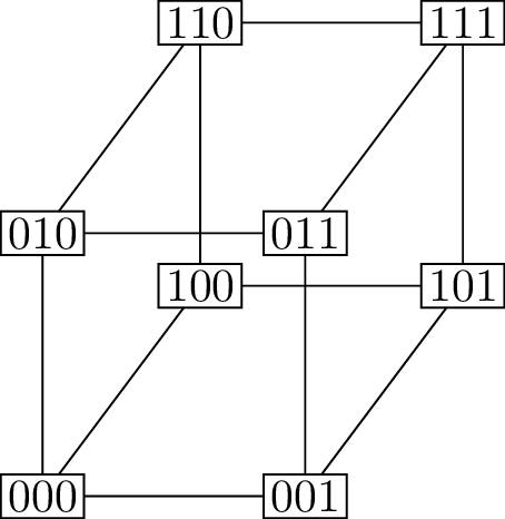
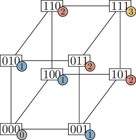
The cube graph \(Q_3\)A \(6\)-cycle in \(Q_3\)A Hamilton cycle in \(Q_3\)
The cube graph and some cycles in it
Suppose that instead of flipping two cups at a time in the three cups
puzzle, we could flip any one cup; the puzzle is no longer challenging
in any way, but it is more interesting as a mathematical object. So we
abandon cups; instead of using the symbols \(\sqcup\) and \(\sqcap\), we switch to the symbols \(0\) and \(1\), so that the vertices are \(3\)-bit sequences. The resulting graph is
shown in Figure 3.3(a). It is called the cube
graph because, in addition to the combinatorial description, it has
a geometric one: the corners and (geometric) edges of the unit cube
\([0,1]^3\) are exactly the vertices
and edges of the cube graph.
We use the notation \(Q_3\) for the
cube graph because in Chapter 4, we
will generalize this graph to the hypercube graph\(Q_n\), with a geometric interpretation in
\(n\) dimensions.
In terms of \(n\), how many vertices does \(Q_n\) have?
\(2^n\)
vertices: there are \(2^n\) sequences
of \(n\) bits, because there are \(2\) choices (\(0\) or \(1\)) for each bit.
The shortest cycles found in \(Q_3\)
have \(4\) vertices, such as the cycle
represented by the closed walk \((000, 001,
011, 010, 000)\). We also have \(6\)-vertex cycles such as the one shown in
Figure 3.3(b): this one is represented by
the closed walk \((000, 010, 110, 111, 101,
001, 000)\). There are even cycles through all \(8\) vertices such as the one represented by
\((000, 001, 011, 010, 110, 111, 101, 100,
000)\), which is shown in Figure 3.3(c). A
cycle through all the vertices of a graph has a special name: it is
called a Hamilton cycle. We will study these in more detail in
Chapter 17.
Lengths of walks
Finally, once we know that an \(x-y\) walk exists, we ask: how many steps
does it need to have?
Definition 3.5. A walk \((x_0, x_1, x_2, \dots, x_l)\) has
length\(l\). We also
say that a path or cycle has length \(l\) if it is represented by a walk of
length \(l\).
This is one of two possible definitions: it counts the edges used by
the walk, but we could also have counted the vertices. We choose to
count the edges because it makes more sense: the walk that goes nowhere
has length \(0\), and in an application
where the walk is a sequence of steps taken (such as in a puzzle), the
length of a walk is the number of steps required.
One slightly strange consequence is that while the cycle graph \(C_n\) has length \(n\), the path graph \(P_n\) has length \(n-1\). For this reason, some authors define
\(P_n\) to be a path with \(n+1\) vertices and \(n\) edges. In my opinion, this causes more
problems than it solves: I am happier if graph families like \(K_n\), \(C_n\), \(P_n\) and others are indexed by the number
of vertices they have, whenever possible.
The main reason to define the length of a walk is so that we can look
for a shortest \(x-y\) walk, avoiding
walking back and forth inefficiently. Walks that don’t revisit any
vertices are exactly the ones that correspond to paths, and in fact,
that is how we will prove Theorem 3.1:
that a graph has an \(x-y\) walk if and
only if it has an \(x-y\) path.
Proof of Theorem 3.1. If a graph \(G\) has an \(x-y\) path, the walk representing it is an
\(x-y\) walk, which proves one
direction of the theorem.
For the other direction, suppose \(G\) has an \(x-y\) walk. In that case, let \((u_0, u_1, \dots, u_l)\), with \(u_0 = x\) and \(u_l = y\), be an \(x-y\) walk of the smallest length possible.
We will show that this walk represents a path.
Suppose not, for the sake of contradiction. If the walk fails to
represent a path, then the vertices are not all distinct, which means we
can pick two positions \(i\) and \(j\) with \(i<j\) such that \(u_i = u_j\). But now, consider the sequence
\[(u_0, u_1, \dots, u_{i-1}, u_i, u_{j+1},
\dots, u_l)\] in which we skip vertices \(u_{i+1}, u_{i+2}, \dots, u_j\). This is
still an \(x-y\) walk! It still starts
at \(x\), still ends at \(y\), and every two consecutive vertices are
adjacent because they were also adjacent in the original walk. (This is
not obvious for the pair \(\{u_i,
u_{j+1}\}\), but because \(u_i =
u_j\), it is the same as the pair \(\{u_j, u_{j+1}\}\).)
So we’ve found an \(x-y\) walk which
has length \(l-(j-i)\): strictly less
than \(l\). This contradicts our
assumption that we took an \(x-y\) walk
of the smallest length possible. So a shortest \(x-y\) walk cannot have repeated vertices:
it must represent an \(x-y\)
path. ◻
We are now in a position where we can measure distances in a graph,
by the lengths of walks connecting them. This is a graph-theoretic
distance, not a geometric one: even if there is a way to measure
distances between vertices of a graph \(G\) geometrically, this might disagree from
the graph-theoretic measure.
For example, imagine a graph defined on the streets in a city by
placing vertices at points \(1\) meter
apart along every street, and joining vertices along the same street.
The length of a walk in this graph tells us the “walking distance”: how
far we’d have to go along the streets of the city to get from one point
to another. This might be very different from distance between two
points “as the crow flies”, if the points are very close together but
without convenient streets between them. It is the “walking distance”,
and its generalizations to other situations, that we use to define
distance between vertices in a graph.
Definition 3.6. The distance
between two vertices \(x\) and \(y\) in a graph \(G\) (sometimes written \(d_G(x,y)\), or \(d(x,y)\) if the graph is clear from
context) is the length of the shortest \(x-y\) walk, which we now know is also the
length of the shortest \(x-y\)
path.
If \(x\) and \(y\) are in different connected components,
then there is no such walk, and we sometimes say that \(d(x,y) = \infty\) in that case.
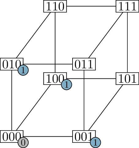
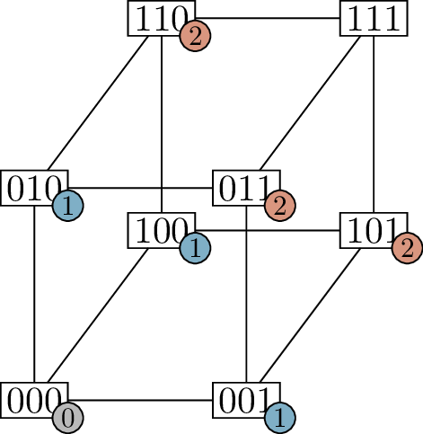
For example, in Figure 3.4(c), all
vertices of the cube graph \(Q_3\) have
been labeled with their distance to the bottom left vertex, \(000\). Take note of the label \(0\) on vertex \(000\) itself. This is
there because vertex \(000\) has
distance \(0\) to itself, as measured
by the length-\(0\) walk \((000)\).
Step 1Step 2Step 3
Finding distances in the cube graph
What’s going on in the other parts of Figure 3.4? These are illustrations of
the steps of an algorithm by which all the distances from a single
vertex may be computed.
Let \(x\) be that starting vertex,
in an arbitrary graph \(G\). We begin
by knowing only one distance in \(G\):
the distance \(d(x,x)=0\).
In Step 1, we take all the neighbors of \(x\); for each vertex \(y\) adjacent to \(x\), we set \(d(x,y)=1\). This is the correct distance,
because the walk \((x,y)\) has length
\(1\), and there cannot be a
length-\(0\) walk from \(x\) to any vertex other than \(x\). Moreover, all length-\(1\) walks from \(x\) end at a neighbor from \(x\), so we’ve found all the vertices at
distance \(1\); this will be important
later. The end result of Step 1 when \(G =
Q_3\) is shown in Figure 3.4(b).
From then on, we repeat the following procedure, of which our Step 1
is a special case. In Step \(k\), we
consider every vertex \(y\) for which
\(d(x,y)=k-1\), and every neighbor
\(z\) of such a vertex for which \(d(x,z)\) is still unknown; we set \(d(x,z)=k\). Why is this correct? There’s
two parts to the verification:
First of all, there is an \(x-z\) walk of length \(k\). To find it, take the \(x-y\) walk of length \(k-1\) (which must exist, assuming the
previous steps of our algorithm were correct) and append vertex \(z\) to the end of that sequence.
Second, there are no shorter \(x-z\) walks; that’s because, at step \(k-1\), we found all the vertices at
distance at most \(k-1\) from \(x\).
Now let’s re-confirm point 2 above for Step \(k\), so we can use it in future steps.
Suppose that \(d(x,z) \le k\); then for
some \(j \le k\), there is a walk \((x_0, x_1, \dots, x_j)\) with \(x_0 = x\) and \(x_j = z\). The walk \((x_0, x_1, \dots, x_{j-1})\) has length
\(j-1\), so \(d(x, x_{j-1}) \le j-1\), and we’ve found
vertex \(x_{j-1}\) at Step \(j-1\) or earlier: before Step \(k\). Finally, in the next step after we
computed \(d(x, x_{j-1})\), we would
have considered \(z\) (a neighbor of
\(x_{j-1}\)), and determined \(d(x, z)\).
In the cube graph \(Q_3\), the
result of Step 2 is shown in Figure 3.4(b) and
the result of Step 3 is shown in Figure 3.4(c).
Here, if we were to try to do a Step 4, we would accomplish nothing: all
neighbors of the vertex labeled with \(3\) already have known distances. At this
point, we stop.
This stopping condition is guaranteed to happen in an \(n\)-vertex graph by Step \(n-1\) or earlier: if we were to do more
steps than that while computing a new distance at every step, we’d run
out of distances to compute. (This is an important thing to check about
every algorithm—that it halts!) After the stopping condition is reached,
let \(S\) be the set of all vertices
whose distances to \(x\) we’ve
computed. There is a walk between any two vertices in \(S\), because all of them have a walk to
\(x\); however, no vertex \(y \in S\) has a neighbor \(z \notin S\), because we would have
computed the value of \(d(x,z)\) a step
after computing \(d(x,y)\) if not
earlier.
Therefore \(G[S]\) is the connected
component of \(G\) containing \(x\). If \(G\) is connected, then we’ve computed all
distances, and we’re done. Otherwise, we can set \(d(x,y)\) to \(\infty\) for all \(y \notin S\).
Is there an \(n\)-vertex graph for which this algorithm
doesn’t stop before Step \(n-1\)?
Yes: the path graph \(P_n\), if we start measuring distances from
one end of the path graph. In this graph, it takes \(n-1\) steps to go from one end to the
other.
This distance-finding algorithm is a special instance of
breadth-first search, or BFS for short. It is a way of exploring the
graph to eventually visit all the vertices in a connected component.
It’s called “breadth-first” because it tries to go outward from the
starting vertex in every direction at once: first a little bit, then a
little bit more, and so on.
In the distance-finding algorithm, we used a breadth-first search to
compute distances, but this algorithm can be used for other purposes as
well; Edward Moore, one of the first people to discover it, used it to
find the shortest path through a maze [74]. Later on in the book, we will see other
problems that can be solved using a similar algorithm.
Practice problems
Let \(G\) be the graph whose
vertices are the numbers \(1, \dots,
15\), with an edge between \(a\)
and \(b\) if \(|a-b|=4\) or if \(|a-b|=10\). (For example, vertex 11 is
adjacent to vertices 7 and 15, because \(|11-7|=|11-15|=4\), as well as to vertex
\(1\), because \(|11-1|=10\).
Draw a diagram of \(G\).
What are the connected components of \(G\)?
Draw a diagram of the circulant graph \(\operatorname{Ci}_{10}(1,3)\).
Choose any vertex of \(\operatorname{Ci}_{10}(1,3)\), and use the
distance-finding algorithm to label every vertex with its distance from
your chosen vertex.
The graph \(\operatorname{Ci}_{10}(1,3)\) has cycles of
four different lengths. What are they? Give an example of each. As a
stretch goal, prove that there are no cycles of other lengths; if you do
not figure out how, see Chapter 13.
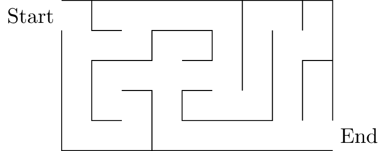
How can we find the shortest path through a maze, as Edward Moore
did, by using breadth-first search on a graph? Try it out on the maze
below:
Suppose we generalize the \(3\)-cup puzzle to an \(n\)-cup puzzle, where a valid move is to
take any two cups that are next to each other and flip them over. Prove
that from any starting state with an even number of cups placed right
side up, it is possible to reach the state where all \(n\) cups are upside down.
Prove that the distance between vertices in a connected graph
satisfies the following properties, for all vertices \(x\), \(y\), and sometimes \(z\):
\(d(x,y) = 0\) if and only if
\(x=y\).
\(d(x,y) = d(y,x)\).
\(d(x,z) \le d(x,y) +
d(y,z)\).
Some of these properties are easier than others, but I am listing
them for two reasons. First of all, in some way, they correspond to the
proof of Lemma 3.3. Second, they are the three
properties that make a connected graph a metric space with metric \(d\); this is not something I will cover in
this textbook, but it is interesting in a context outside graph
theory.
To really understand the proof of Lemma 3.3, it helps to try to generalize
it and see what works and what doesn’t. Take the following two relations
on the vertices of a graph \(G\):
\(x \frown y\) if there is a
\(x - y\) walk of odd length.
\(x \smile y\) if there is a
\(x - y\) walk of even length.
For one of these, we can copy the proof of Lemma 3.3 almost word-for-word and prove
that it is also an equivalence relation. For the other one, this will
not work: there are two places where the proof will fail. Find those
places!
(Putnam 2010) There are \(2010\)
boxes labeled \(B_1, B_2, \dots,
B_{2010}\), and \(2010n\) balls
have been distributed among them, for some positive integer \(n\). You may redistribute the balls by a
sequence of moves, each of which consists of choosing an \(i\) and moving exactly \(i\) balls from box \(B_i\) into any one other box. For which
values of \(n\) is it possible to reach
the distribution with exactly \(n\)
balls in each box, regardless of the initial distribution of
balls?
(IMO 1991) Suppose \(G\) is a
connected graph with \(k\) edges. Prove
that it is possible to label the edges \(1, 2,
\dots, k\) in such a way that at each vertex which belongs to two
or more edges, the greatest common divisor of the integers labeling
those edges is \(1\).
Footnotes
To make the puzzle appear possible to solve, you can do
the following: set up the puzzle in the alternating \(\sqcup\sqcap\sqcup\) state, and make a few
moves back and forth before arriving at the desired \(\sqcap\sqcap\sqcap\). Then explain that
you’re “resetting” the puzzle, and bring it back to an alternating state
before letting your victim try solving it—but make it, instead, the
\(\sqcap\sqcup\sqcap\) state. After
this, the puzzle will be impossible. You can further disguise the nature
of the puzzle by using \(5\) cups
instead of \(3\).↩︎
Keep in mind that this is not quite the same as joining
the sequences together: the last vertex of the \(x-y\) walk and the first vertex of the
\(y-z\) walk are both \(y\), and only one of those \(y\)’s should be kept in the \(x-z\) walk.↩︎