It is a little strange of me to put the chapter on line graphs in the
part of the textbook devoted to hard problems, because there is not
really a hard problem associated to line graphs. The opposite is true:
the hard problems in this section are often easier to solve when we are
solving them in a line graph. And that’s exactly why I think these
chapters belong together!
By looking at line graphs, we will also see many connections between
problems that seemed very different before. There is an occasionally
useful relationship between Euler tours (Chapter 8) in a
graph \(G\) and Hamilton cycles
(Chapter 17) in its line graph \(L(G)\). Matchings (Chapter 13 through Chapter 16) are exactly the same thing as
independent sets (Chapter 18)
in the line graph. And by extending graph coloring to line graphs, we
will arrive at edge coloring, a new problem with its own
applications.
You can see from this list that to understand all the material in
this chapter, you need to be familiar with many concepts in previous
parts of the textbook. Apart from the chapters mentioned above, you
should be familiar with Chapter 7, because both
directed graphs and multigraphs will make an appearance.
It is not necessarily the case that you want to read the entire
chapter if you’re learning graph theory for the first time (or to teach
the entire chapter in an introductory course). The application to de
Bruijn sequences is interesting, but self-contained. Vizing’s theorem is
a natural observation to make after observing enough examples, but
difficult to prove, though I have tried to pick out a less complicated
proof.
Line graphs
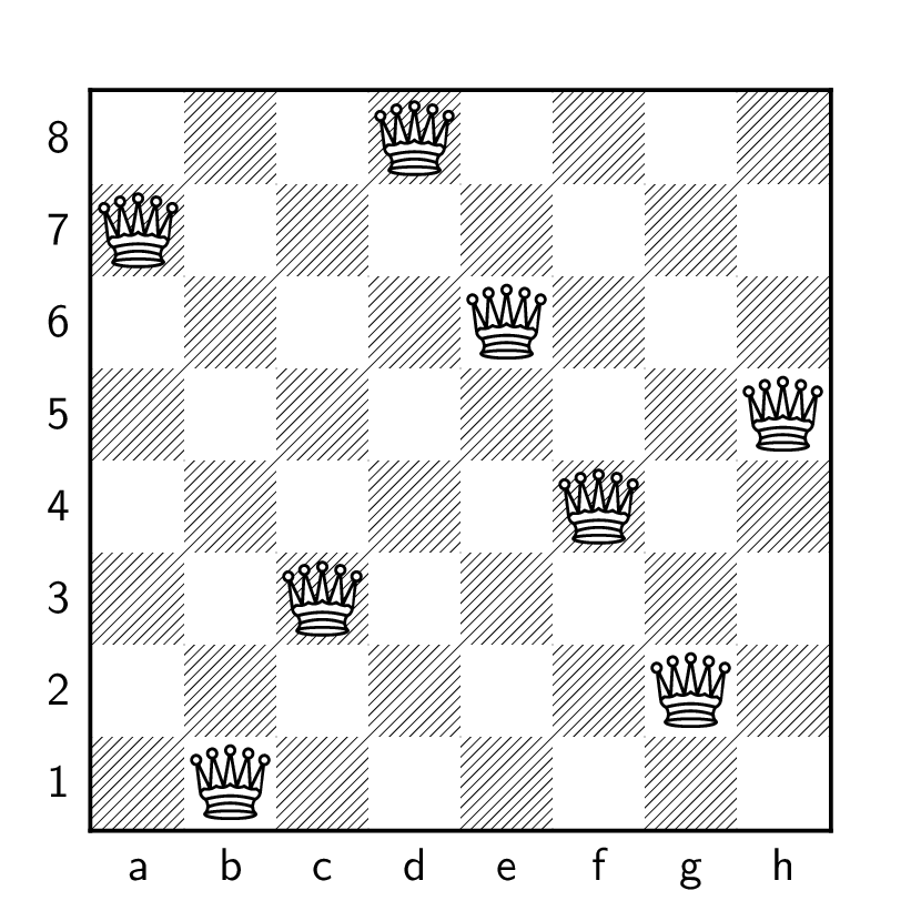
Eight queens: an independent setEight rooks: a… matching?
Rook and queen placements
In Chapter 13 and Chapter 18, I used two very similar
problems as an example: the problem of placing eight rooks on a
chessboard, and the problem of placing eight queens on a chessboard, so
that they do not attack each other. The solutions are shown once again
in Figure 20.1, for your reference. (Of
course, the eight queens problem is strictly harder than the eight rooks
problem, because a queen has all the movement power of a rook and more,
so instead of Figure 20.1(b), we
could have just taken Figure 20.1(a) and changed all the
queens to rooks.)
However, there’s something strange about how we modeled these
problems. The eight queens problem was our first example of finding
independent sets in a graph: a hard problem we have no good algorithms
for. It would have been equally natural to try solving the eight rooks
problem in the same way. Define the \(8\times 8\) rook graph to be the graph
whose \(64\) vertices are the squares
of a chessboard, with an edge between two squares which are in the same
rank or file. Then a solution to the eight rooks problem is an
independent set in the \(8\times 8\)
rook graph.
We did something different in Chapter 13—and a good thing, too!
Instead of finding an independent set, we were able to solve the problem
by finding a matching, which is much easier. But why is it that the
eight rooks problem has these two different models, and what is the
relationship between them?
The answer is: the \(8\times 8\)
rook graph happens to be a line graph, whose special structure makes
many problems easier.
Definition 20.1. The line graph\(L(G)\) of a graph \(G\) is the graph whose vertices are the
edges of \(G\); two vertices \(e, e'\) of \(L(G)\) are adjacent if and only if edges
\(e\) and \(e'\) share an endpoint in \(G\).
Why is this the “line” graph? The name was introduced by Frank Harary
and Robert Norman in 1960 [50], who referred to the vertices and edges of
graphs as “points” and “lines”. As a result, Harary and Norman called
\(L(G)\) the line graph because its
vertex set (or “point set”) was the set of “lines” of \(G\). The name stuck.
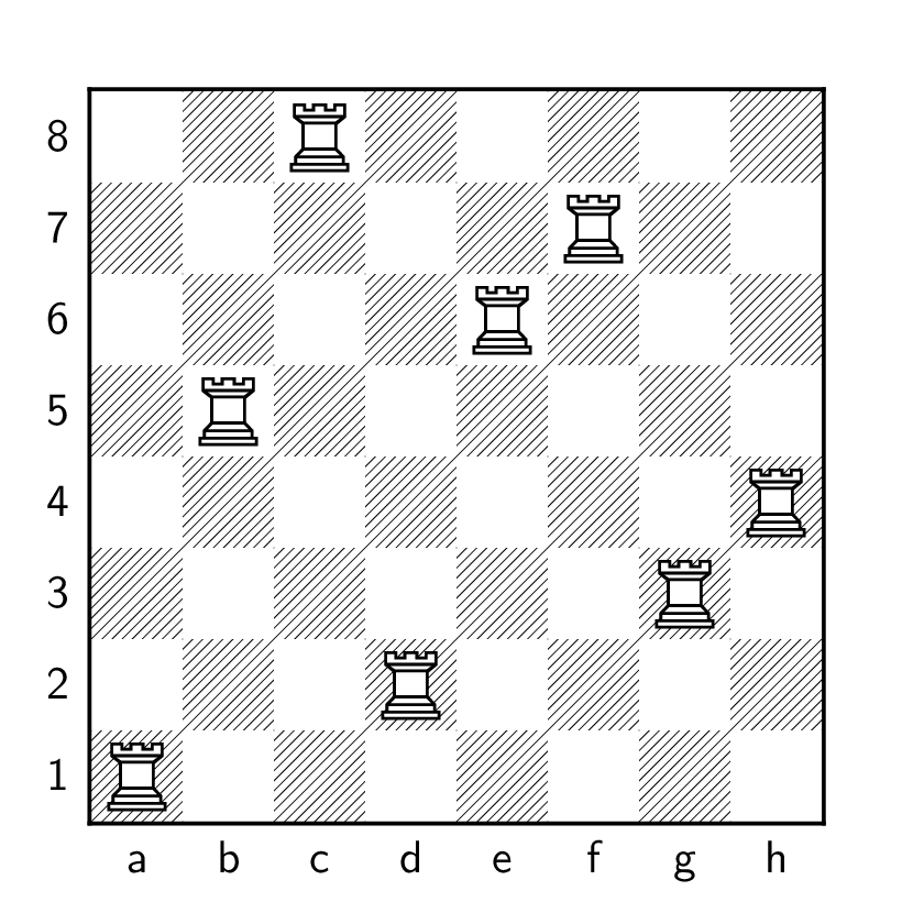
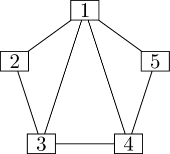
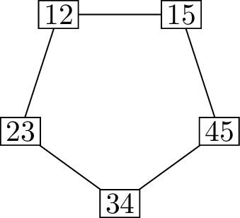
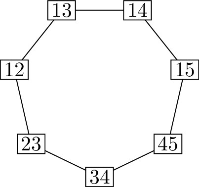
Let’s look at some examples. Figure 20.2(a) and
Figure 20.2(b) show a graph \(G\) with nothing particularly special about
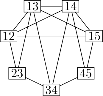
it, and its line graph \(L(G)\). The
line graph has \(7\) vertices, which
correspond to the \(7\) edges of \(G\). Observe what happens to the four edges
\(12\), \(13\), \(14\), and \(15\) incident to vertex \(5\): they turn into a \(4\)-vertex clique in \(L(G)\).
\(G\)\(L(G)\)\(L(C_5)\)\(L(K_{3,3})\)
Several examples of line graphs
Most graphs have line graphs that are bigger than they are in every
way, but not all. For example, Figure 20.2(c)
shows the line graph of \(C_5\): we see
that \(L(C_5)\) is isomorphic to \(C_5\) itself, and the same will happen for
every cycle graph.
What is the line graph of a path graph
\(P_n\) isomorphic to?
\(L(P_n)\) is isomorphic to \(P_{n-1}\): an \(n\)-vertex path has \(n-1\) edges, each sharing an endpoint with
the previous edge and the next edge along the path.
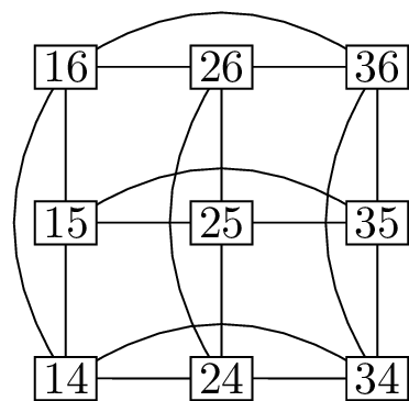
Finally, Figure 20.2(d)
shows the line graph of the complete bipartite graph \(K_{3,3}\) (with vertices \(\{1,2,3\}\) on one side and \(\{4,5,6\}\) on the other side of the
bipartition). It is also isomorphic to the \(3
\times 3\) rook graph, showing the possible moves a rook could
make on a \(3\times 3\) chessboard.
With a little imagination, this should let you see how the \(8\times 8\) rook graph is isomorphic to the
line graph \(L(K_{8,8})\).
It is also possible to define the line digraph of a directed graph;
the idea is similar, but two arcs that share an endpoint will only
correspond to an arc in the line digraph when their orientations are
compatible.
Definition 20.2. The line
digraph\(L(D)\) of a directed
graph \(D\) is the directed graph whose
vertices are the arcs of \(D\). For
every pair of arcs \((x,y)\) and \((y,z)\) in \(D\) such that the first arc ends where the
second arc starts, there is an arc \(\big((x,y), (y,z)\big)\) in \(L(D)\).
It often turns out that one problem in graph theory is equivalent to
another problem in disguise: solving one problem in the graph \(G\) is equivalent to solving the other in
\(L(G)\). Even when these are not
exactly equivalent, the relationship can help us understand both
problems better.
For example, as we see in the case of the eight rooks problem,
finding a matching in a graph \(G\) is
equivalent to finding an independent set in \(L(G)\). A matching in \(G\) is a set of edges such that no two
edges share an endpoint. A set of edges in \(G\) is precisely a set of vertices in \(L(G)\), and sharing an endpoint is
precisely what defines adjacency in \(L(G)\). Therefore a set \(M \subseteq E(G)\) is a matching in \(G\) if and only if it is an independent set
in \(G\).
The notation that we’ve used for the two problems is suggestive of
this relationship: we used \(\alpha(G)\) to denote the independence
number of \(G\), and \(\alpha'(G)\) to denote the matching
number. We could already have said the vague phrase, “\(\alpha'(G)\) is the edge version of
\(\alpha(G)\)”. Now we can make this
precise: \(\alpha'(G) =
\alpha(L(G))\).
Beyond this example, it is often the case that a numerical graph
invariant \(f(G)\) will be given an
edge version \(f'(G)\), defined as
\(f(L(G))\). Unfortunately, sometimes,
an invariant will also be written \(f'(G)\) if it gives off vague vibes of
being the edge version of \(f(G)\),
even if it is not always equal to \(f(L(G))\). You should be careful and check
if \(f'(G) = f(L(G))\) holds when
faced with new notation; don’t just assume it.
What do cliques in \(L(G)\) correspond to?
With one exception, a set of vertices in
\(L(G)\) is a clique when those
vertices are edges in \(G\) that all
share a common endpoint. If it weren’t for that pesky exception, we
could think of the maximum degree \(\Delta(G)\) as being an “edge clique
number” \(\omega'(G)\)…
What’s the pesky exception?
There’s another way for vertices in \(L(G)\) to form a clique: if they correspond
to the three edges of a cycle of length \(3\). Thus, if \(G\) is a graph with maximum degree \(2\), but one connected component of \(G\) is a cycle of length \(3\), then \(\omega(L(G))\) will be \(3\), not \(2\).
The benefit of identifying the matching number \(\alpha'(G)\) as \(\alpha(L(G))\) is that it makes the problem
of finding an independent set easier in a line graph. If we identify a
graph \(H\) as being isomorphic to
\(L(G)\) for some \(G\), then we can reduce the hard problem of
finding \(\alpha(H)\) to the easier
problem of finding \(\alpha'(G)\).
Euler tours and Hamilton
cycles
An Euler tour in a graph is a closed walk that uses each edge exactly
once. A Hamilton cycle in a graph is a cycle that uses each vertex
exactly once. When the descriptions of two problems match so closely,
but one uses “vertex” where the other uses “edge”, it is natural to
suspect that line graphs could be involved.
In fact, half of a relationship is present. We can prove the
following result:
Proposition 20.1. Every Euler tour in a graph
\(G\) corresponds to a Hamilton cycle
in \(L(G)\).
Proof. Suppose that the closed walk \((x_0, x_1, x_2, \dots, x_m)\), with \(x_m=x_0\), is an Euler tour in \(G\). Then consider the following sequence
of edges of \(G\) (or vertices of \(L(G)\)): \[(x_0
x_1, x_1x_2, x_2x_3, \dots, x_{m-1}x_m, x_mx_0, x_0x_1).\] These
are, in fact, edges of \(G\), because
they are pairs of consecutive vertices of the closed walk. In fact, by
the definition of an Euler tour, if we leave out the last element of
this sequence (which is the same as the first element), then every edge
of \(G\) is included exactly once.
Finally, two consecutive edges in this sequence have the form \(xy, yz\), and share an endpoint: so they
are adjacent in \(L(G)\). These are
exactly the conditions needed to be certain that this sequence is a
closed walk representing a Hamilton cycle in \(L(G)\). ◻
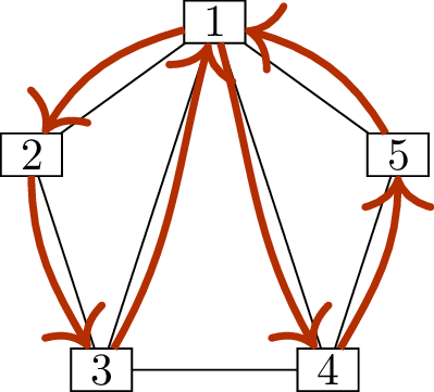
A walk with no repeated edgesThe corresponding \(6\)-cycleA Hamilton cycle in \(L(G)\)
Euler tours in \(G\) and
Hamilton cycles in \(L(G)\)
Figure 20.3 shows a partial
illustration of this principle, using as an example the graph \(G\) from Figure 20.2(a),
whose line graph was shown in Figure 20.2(b).
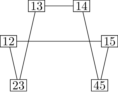
The closed walk in Figure 20.3(a)
is not an Euler tour, but it is a closed walk with no repeated edges, so
it shares most of the same properties. We can apply the same
transformation \[(1,2,3,1,4,5,1) \leadsto
(12, 23, 13, 14, 45, 15, 12)\] as we did in the proof of
Proposition 20.1. (I have adjusted the
order in which an edge is written, in some cases, so that it matches how
Figure 20.3(b) is labeled.)
What can the argument of Proposition 20.1 tell us if we apply it
to closed walks like this one, which use each edge at most once?
The resulting closed walk in \(L(G)\) represents a cycle, but not
necessarily a Hamilton cycle. Here, the original walk did not use the
edge \(34\), and so vertex \(34\) is not part of the cycle.
Figure 20.3(c), on the other hand, shows a
Hamilton cycle in \(L(G)\). We should
be suspicious of this, because the original graph \(G\) is not Eulerian: vertices \(3\) and \(4\) have odd degree! And, in fact, the
converse to Proposition 20.1 is false: Hamilton
cycles in \(L(G)\) do not always
correspond to Euler tours in \(G\).
What went wrong?
When visiting vertices \(15, 14, 13, 12\) in \(L(G)\), though they all share an endpoint,
they all share the same endpoint. To continue a walk in \(G\), it is not enough to know which edge
was the last edge used; we need to know which of its endpoints was the
last vertex used, to continue from that vertex.
This problem goes away if we consider directed graphs and their line
digraphs. If \(a, a'\) are two arcs
in a directed graph \(D\), then the
line digraph \(L(D)\) can afford to be
pickier about when it has an arc \((a,a')\). The arc \((a,a')\) is not just included when
\(a\) shares an endpoint with \(a'\), but when they share endpoints
compatibly: when \(a\) ends where \(a'\) starts. This lets us prove the
following:
Proposition 20.2. If \(D\) is a directed graph, then Euler tours
in \(D\) correspond to Hamilton cycles
in \(L(D)\), and vice versa.
Proof. I will omit the proof that an Euler tour in \(D\) corresponds to a Hamilton cycle in
\(L(D)\), because the argument is the
same as in Proposition 20.1.
Suppose that in \(L(D)\), we have a
Hamilton cycle represented by the walk \[(a_0, a_1, \dots, a_{m-1}, a_0).\] For
each \(i=0, 1, \dots, {m-1}\), let
\(a_i = (x_i, y_i)\), and consider the
sequence \[T = (x_0, x_1, \dots, x_{m-1},
x_0)\] of vertices in \(D\).
For each \(i=0, 1, \dots, m-1\),
there must be an arc \((a_i, a_{i+1})\)
in \(L(D)\), meaning that \(y_i = x_{i+1}\). Therefore there is an arc
\((x_i, x_{i+1})\) in \(D\): this is another way to write the arc
\(a_i\). Similarly, there is an arc
\((a_{m-1}, a_0)\) in \(L(D)\), so \(y_{m-1} = x_0\), and therefore \(D\) has the arc \((x_{m-1}, x_0)\). This means that \(T\) is a walk in \(D\).
The arcs used by \(T\) are precisely
the arcs \(a_0, a_1, \dots, a_{m-1}\),
in that order. Since we started with a Hamilton cycle in \(L(D)\), these arcs include each vertex of
\(L(D)\) exactly once, so they include
each arc of \(D\) exactly once.
Therefore \(T\) is an Euler tour. ◻
We solved the problem of finding Euler tours completely in Chapter 8, while the problem of finding
Hamilton cycles is difficult and remains difficult in directed graphs.
This means that if we spot that a certain directed graph happens to be a
line digraph, we can make use of this to turn a difficult problem into
an easy problem.
De Bruijn sequences
This happens, for example, in the study of de Bruijn sequences. To
introduce these, let me give an example: the sequence \[\mathsf{aabaacabbabcacbaccbbbcbccca},\]
which you should think of as being cyclic: when you get to the end, keep
reading again from the start.1 A \(3\)-letter substring of this
sequence is what you get if you start anywhere and read the next \(3\) letters: for example, you could start
at the beginning, you will get aab, or
start at the first c and get cab. There are \(27\) letters in the sequence, so there are
\(27\) possible substrings; the magical
property of this sequence is that every possible substring occurs
exactly once.
Where does the substring aaa occur?
You must start at the last character,
reading an a and then reading aa from the beginning.
In general, given an alphabet \(A\)
(any set of symbols) and a positive integer \(n\), we can define the de Bruijn
sequence of order \(n\) over \(A\) to be a cyclic sequence with the same
property: its length-\(n\) substrings
contain every possible substring exactly once. Of course, we can define
anything we like, but that’s no guarantee that such a thing exists!
These sequences are named after Nicolaas Govert de Bruijn, who proved
in 1946 [11] that they
exist: for all \(n\) and all alphabets
\(A\). To do this, de Bruijn used graph
theory; but what is the right graph model for this problem?
One extreme option is to use \(A\)
as the set of vertices, putting every possible edge between them, so
that a de Bruijn sequence is a particular kind of closed walk in the
graph. Such an approach is almost never the right choice, and it is not
the right choice here. The problem is that the graph we get doesn’t
manage to encode the rules of the problem in any way: we don’t benefit
from looking at the problem with the graph in mind. Ideally, once we
build the graph that describes the problem, the solution should be some
very standard object inside that graph.
Another option is to take our vertices to be the set of all \(|A|^n\) of the \(n\)-symbol strings that we want to see
inside the de Brujin sequence. It is still tempting to have the de
Bruijn sequence be a closed walk in the graph we define. To make this
happen, we need the edges to answer the question: if string \(x\) is the \(n\)-symbol string at position \(i\) in the sequence, which strings could
start at position \(i+1\)?
Suppose that reading from position \(i\), we see the symbol \(x_0 x_1 \dots x_{n-1}\). What strings could
we see, reading from position \(i+1\)?
We could see any of the sequences of the
form \(x_1 x_2 \dots x_n\), where \(x_n \in A\) could be any symbol.
This is an asymmetric relationship, so we define a directed graph
with all vertices of the form \(x_0 x_1 \dots
x_{n-1}\) and all arcs of the form \((x_0 x_1 \dots x_{n-1}, x_1 x_2 \dots
x_n)\).
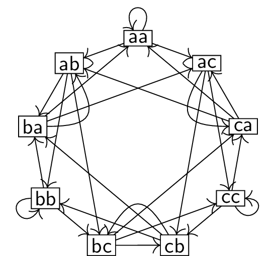
We call this directed graph the de Brujin digraph; the
notation \(B(k,n)\) is sometimes used
for the de Bruijn digraph for strings of order \(n\) with a \(k\)-symbol alphabet. (Up to isomorphism of
the graph, it does not matter what the alphabet is.) An example is shown
in Figure 20.4(a). I have kept \(A = \{\mathsf a, \mathsf b, \mathsf c\}\),
but to avoid making this graph too large, I have reduced \(n\) to \(2\).
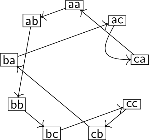
Unfortunately, there’s a problem. If we want to find a de Bruijn
sequence of order \(n\) in the graph
\(B(k,n)\), we must find a Hamilton
cycle in the graph, because we want to visit every vertex. Figure 20.4(b) shows such a cycle in \(B(3,2)\). This gives us the de Bruijn
sequence aabbccbac… but at what cost?
Finding Hamilton cycles is very difficult, so we might as well have
brute-forced the problem.
A diagram of \(B(3,2)\)A Hamilton cycle in \(B(3,2)\)An Euler tour in \(B(3,1)\)
Approaches to solving the de Bruijn sequence
problems
The trick is to realize the following incredibly convenient
coincidence:
Proposition 20.3. For all \(k \ge 1\) and \(n\ge 2\), the de Bruijn digraph \(B(k,n)\) is isomorphic to the line digraph
of \(B(k,n-1)\).
Proof. To find an isomorphism between \(L(B(k,n-1))\) and \(B(k,n)\), we need a function \(\varphi\) from the vertices of \(L(B(k,n-1))\) (or the arcs of \(B(k,n-1)\)) to the vertices of \(B(k,n)\).
An arc in \(B(k,n-1)\) is a pair
\((x_0 x_1 \dots x_{n-2}, x_1 x_2 \dots
x_{n-1})\), where \(x_0, x_1, \dots,
x_{n-1} \in A\). Since the vertices of \(B(k,n)\) are also defined by \(n\) symbols from \(A\), the natural thing to try is to define
\[\varphi\Big((x_0 x_1 \dots x_{n-2}, x_1 x_2
\dots x_{n-1})\Big) = x_0 x_1 \dots x_{n-1}\] and see if this
works.
What does it mean for \(\varphi\) to work: what will make it an
isomorphism?
We need to check if \(\varphi\) preserves arcs: we want \((x,y)\) to be an arc in \(L(B(k,n-1))\) if and only if \((\varphi(x), \varphi(y))\) is an arc in
\(B(k,n)\).
Take two vertices in \(L(B(k,n-1))\): let one vertex be the pair
\((x_0 x_1 \dots x_{n-2}, x_1 x_2 \dots
x_{n-1})\), and let the other be the pair \((y_0 y_1 \dots y_{n-2}, y_1 y_2 \dots
y_{n-1})\). There is an arc from the first two the second exactly
when \(x_1 x_2 \dots x_{n-1} = y_0 y_1 \dots
y_{n-2}\), by the definition of a line graph.
Now apply \(\varphi\) to both
vertices: we get \(x_0x_1\dots
x_{n-1}\) and \(y_0 y_1 \dots
y_{n-1}\). By the definition of \(B(n,k)\), there is an arc from the first to
the second exactly when \(x_1 x_2 \dots
x_{n-1} = y_0 y_1 \dots y_{n-2}\): the same condition!
Therefore \(\varphi\) really is an
isomorphism, completing the proof. ◻
Instead of a Hamilton cycle in \(B(k,n)\), we can look for an Euler tour in
\(B(k,n-1)\), which is much
easier.
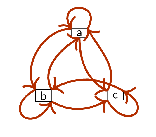
For example, Figure 20.4(c)
shows the same de Bruijn sequence aabbccbac, but this time it is obtained from
an Euler tour in \(B(3,1)\). (It’s very
hard to show Euler tours in a diagram; here, different visits to the
same vertex touch it at different points. To obtain aabbccbac, start at the northeast corner of
vertex a and follow the arrows.)
Theorem 20.4. For any set of symbols \(A\) and any integer \(n\ge 1\), there is a de Bruijn sequence of
order \(n\) over \(A\).
Proof. For \(n=1\), just
write all the symbols in \(A\), one
after the other.
For \(n\ge 2\), we must prove that
the digraph \(B(k,n-1)\) is Eulerian,
where \(|A|=k\). By Corollary 8.6, we
must check two properties of \(B(k,n-1)\). (Both properties were defined
in Chapter 8.)
First, we check that \(B(k,n-1)\) is
weakly connected. We can prove this by giving an \(x-y\) walk for any two vertices \(x = x_0 x_1 \dots x_{n-2}\) and \(y = y_0 y_1 \dots y_{n-2}\). One possible
walk passes through all vertices of the form \[\underbrace{x_i x_{i+1} \dots
x_{n-1}x_{n-2}}_{n-2-i \text{ symbols from }x} \underbrace{y_0 y_1 \dots
y_{i-2}y_{i-1}}_{i \text{ symbols from }y}\] for \(i = 0, 1, \dots, n-2\), in that order.
Second, we check that all vertices of \(B(k,n-1)\) are balanced, with
indegree equal to outdegree. In fact, each vertex \(x_0 x_1 \dots x_{n-2}\) has both indegree
and outdegree \(k\): it receives an arc
from every vertex of the form \(x x_0 x_1
\dots x_{n-3}\), where \(x \in
A\), and sends an arc to every vertex of the form \(x_1 x_2 \dots x_{n-2} x\), where \(x \in A\).
Whenever you see that \(n-3\), you should be worried that \(n-3\) is negative. What happens then?
Then, interpret \(x_0 x_1 \dots x_{n-3}\), and for that
matter \(x_1 x_2 \dots x_{n-2}\), as
being empty. When \(n=2\), each vertex
receives an arc from every vertex of the form \(x\), where \(x
\in A\); that is, from every vertex.
By applying Corollary 8.6, we
obtain an Euler tour in \(B(k,n-1)\),
which corresponds to a Hamilton cycle in \(B(k,n)\), which gives us a de Bruijn
sequence of order \(n\). ◻
Edge coloring
So far, we’ve used line graphs to draw connections between ideas
we’ve already seen; now, let’s use them to define something new: the
edge chromatic number. This invariant is also sometimes called the
“chromatic index”; I don’t like this terminology, because there’s
nothing about the words “number” and “index” suggesting that one is
about vertices and the other is about edges.
If \(G\) is a graph, we define the
edge chromatic number \(\chi'(G)\) to be \(\chi(L(G))\): the chromatic number of the
line graph of \(G\). We can also avoid
invoking \(L(G)\), and instead define
\(\chi'(G)\) to be the least number
of colors needed for an edge coloring of \(G\). This is a function \(f\colon E(G) \to C\), where \(C\) is a set of colors, such that each
vertex is incident to at most one edge of each color.2
What are the color classes of an edge
coloring?
The color classes of a vertex coloring of
\(G\) are independent sets in \(G\), so the color classes of an edge
coloring of \(G\) are independent sets
in \(L(G)\): these correspond to
matchings in \(G\).
The upper and lower bounds from the previous chapter can also be used
here: we have \(\omega(G) \le \chi(G) \le
\Delta(G)+1\) for all graphs \(G\), so in particular, \(\omega(L(G)) \le \chi(L(G)) \le \Delta(L(G)) +
1\).
What does \(\omega(L(G)) \le \chi(L(G))\) say, when
translated from \(L(G)\) back to \(G\)?
We’ve already seen that \(\omega(L(G))\) is \(\Delta(G)\), with one exception, and \(\omega(L(G))\ge \Delta(G)\) even then.
Therefore \(\chi'(G) \ge
\Delta(G)\).
What about the upper bound \(\chi(L(G)) \le \Delta(L(G))+1\)?
An edge \(xy\) shares an endpoint with at most \(\Delta(G)-1\) other edges at \(x\), and \(\Delta(G)-1\) more at \(y\); therefore \(xy\) has degree at most \(2 \Delta(G)-2\) in \(L(G)\). We can conclude that \(\chi'(G) \le 2\Delta(G)-1\).
The inequalities \(\Delta(G) \le
\chi'(G) \le 2\Delta(G)-1\) are intriguing: the lower and
upper bound are both in terms of the maximum degree. However, much more
will turn out to be true!
Although the definition of \(\chi'(G)\) is new, we have already seen
one very similar problem already. In Chapter 16, we
looked at \(1\)-factorizations, which
are decompositions of a regular graph into perfect matchings.
If a \(k\)-regular graph \(G\) has a \(1\)-factorization, what does that say about
\(\chi'(G)\)?
We can use the \(1\)-factorization to get an edge coloring
of \(G\), by making each perfect
matchings one of the color classes. There are \(k\) perfect matchings in the \(1\)-factorization, so \(\chi'(G) = k = \Delta(G)\): we already
know this is the minimum possible.
In Chapter 16, we proved two results about
\(1\)-factorizations. Theorem 16.3 says
that for all even \(n\), \(K_n\) has a \(1\)-factorization; this means \(\chi'(K_n) = n-1\) when \(n\) is even. Also, Theorem 16.5
says that every \(k\)-regular bipartite
graph \(G\) has a \(1\)-factorization; this means \(\chi'(G) = k\).
With just a little bit of trickery, we can make the second result
more powerful. Let \(G\) be any
bipartite graph with maximum degree \(\Delta(G)\). There are many ways to find a
bipartite graph \(H\) which contains
\(G\) as a subgraph, and is \(\Delta(G)\)-regular. (I will leave it to
you to discover how to do this, in a practice problem at the end of this
chapter.) Then \(\chi'(H) =
\Delta(G)\), and so in particular \(\chi'(G) = \Delta(G)\): inside every
edge coloring of \(H\), there is an
edge coloring of \(G\). We
conclude:
Corollary 20.5. If \(G\) is any bipartite graph, then \(\chi'(G) = \Delta(G)\).
(This result, in somewhat different terminology, was proven by Kőnig
in 1916 together with Theorem 16.5[62].)
Thus far, we’ve seen many instances where \(\chi'(G) = \Delta(G)\). Is this
universal? No: for example, this will not happen for \(K_n\) when \(n\) is odd. In this case, the largest
matching has only \(\frac{n-1}{2}\)
edges, so it takes at least \(n\)
matchings to cover all \(\frac{n(n-1)}{2}\) edges of \(K_n\). However, Corollary 16.4
says that when \(n\) is odd, \(K_n\) has a decomposition into \(n\) nearly perfect matchings; this means
\(\chi'(K_n) = n\) when \(n\) is odd.
An edge \(4\)-coloring of
the Petersen graphAll edges must have different colors
Two examples of lower bounds on edge coloring
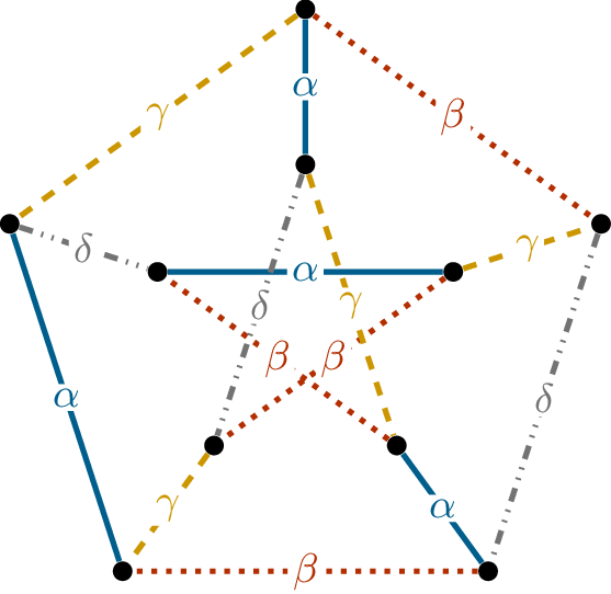
Another interesting example is the Petersen graph. It is \(3\)-regular, and has many perfect
matchings, so you might be tempted to hope that it has edge chromatic
number \(3\). However, this is not
true. Suppose for contradiction that the Petersen graph has an edge
coloring with \(3\) colors \(\{\alpha, \beta, \gamma\}\). (It is
traditional to use Greek letters for the colors of edges; this has
nothing to do with the graph invariants \(\alpha(G)\) or \(\beta(G)\).)
To color all \(15\) edges, each
color class must contain \(5\) edges
and be a perfect matching. If we take the subgraph formed by the edges
with colors \(\alpha\) and \(\beta\), it is \(2\)-regular: each connected component is a
cycle. Moreover, the edges around a cycle must alternate between the
colors \(\alpha\) and \(\beta\), so each component has even
length.
There are two ways to have a \(10\)-vertex graph whose connected
components are cycles of even length: it can be a copy of \(C_{10}\), or the disjoint union of copies
of \(C_4\) and \(C_6\). In the Petersen graph, neither is
possible: the first case contradicts Proposition 17.1,
where we proved that the Petersen graph does not have a Hamilton cycle,
and the second case contradicts Lemma 5.3,
where we proved that it has no cycles of length \(3\) or \(4\). So the Petersen graph cannot have an
edge coloring with only \(3\)
colors.
The Petersen graph does have an edge coloring with \(4\) colors, as shown in Figure 20.5(a). It is
another example of a graph \(G\) with
\(\chi'(G) = \Delta(G)+1\).
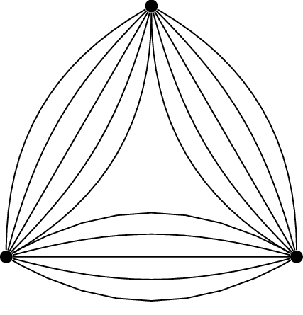
Is this the limit? Not if we consider multigraphs. Figure 20.5(b) shows an example given by
Claude Shannon [91]; in
this multigraph, any two edges share an endpoint, so they must all be
given different colors. If there are \(k\) copies of each edge of the triangle,
then the graph has maximum degree \(2k\), but edge chromatic number \(3k\) (equal to the number of edges).
Shannon also proved that this is the worst case: \(\chi'(G) \le \frac32 \Delta(G)\), even
if \(G\) is a multigraph.
For simple graphs, however, we have only seen examples where \(\chi'(G)\) is either \(\Delta(G)\) or \(\Delta(G)+1\). In 1964, Vadim Vizing proved
that this is true for all simple graphs \(G\)[102]. Since there are only two possible values
of \(\chi'(G)\), sometimes a graph
\(G\) will be referred to as “class
one” if \(\chi'(G) = \Delta(G)\)
and “class two” if \(\chi'(G) =
\Delta(G)+1\).
I will conclude this chapter with a proof of Vizing’s theorem:
Theorem 20.6 (Vizing’s theorem). For all graphs
\(G\), \(\chi'(G) \le \Delta(G)+1\).
Vizing’s theorem
All proofs of Vizing’s theorem that I am aware of rely on a variant
of the alternating paths we used in Chapter 14 or
Chapter 16 when working with matchings.
This makes sense, since a color class in an edge coloring of \(G\) is an independent set in \(L(G)\): a matching in \(G\). However, instead of trying to improve
a single matching, we will be trying to rearrange the existing matchings
to make room for one more edge.
Suppose that \(\alpha\) and \(\beta\) are two of the colors used in an
edge coloring of a graph. The subgraph formed by edges of colors \(\alpha\) and \(\beta\) is the union of two matchings, so
its connected components consist of paths and cycles. A path component
of this subgraph is called an \(\alpha/\beta\)-path.
The colors of the edges of an \(\alpha/\beta\)-path alternate between \(\alpha\) and \(\beta\). If \(x\) is the start or end of an \(\alpha/\beta\)-path, then only one of the
two colors is used on edges incident to \(x\), and it is the edge beginning the \(\alpha/\beta\)-path. Conversely, if only
one of \(\alpha\) or \(\beta\) is used on edges incident to some
vertex \(x\), then we can find an \(\alpha/\beta\)-path starting at \(x\), by greedily following edges of color
\(\alpha\) or \(\beta\) until we cannot continue.
The use of an \(\alpha/\beta\)-path
is that we can swap the colors \(\alpha\) and \(\beta\) on every edge of the path and
obtain a different edge coloring. We can hope to use such a swap to make
color \(\alpha\) or \(\beta\) available for an edge we have not
yet colored.
The proof that follows is based on a proof of Ehrenfeucht, Faber, and
Kierstead [26],
simplified from their more general statement.
Proof of Theorem 20.6. For a fixed number of colors
\(q\), we induct on the number of
vertices in \(G\), proving that if
\(\Delta(G) \le q-1\), then \(G\) has an edge \(q\)-coloring. We can take a \(1\)-vertex graph as our base case, in which
case no edges need to be colored at all. To induct, we take a graph
\(G\) with \(\Delta(G) \le q-1\) and an arbitrary vertex
\(x\), and assume that \(G-x\) has an edge \(q\)-coloring; we must find a way to turn it
into an edge \(q\)-coloring of \(G\).
As we color the edges incident to \(x\) one at a time, we keep a partition of
these edges into three sets \(S \cup T \cup
U\), each with their own meaning:
Edges in \(S\) are
settled, and their color will not change.
There is at most one edge in \(T\), which is tentatively
colored.
Edges in \(U\) are
uncolored.
Our algorithm will maintain the following invariant at all times: the
colors on \(E(G-x) \cup S \cup T\) must
always be an edge coloring of \(G-U\).
When we begin, we put all edges incident to \(x\) in \(U\). These edges have a valuable
flexibility: in \(L(G)\), they have at
most \(\Delta(G)-1\), or \(q-2\), neighbors that have been given a
color, so they have at least \(2\)
colors available to them. To preserve this flexibility, we select two
candidate colors for each edge \(xy
\in U\), satisfying a second invariant. For as long as edge \(xy\) remains in \(U\), it will have two candidate colors,
which must not appear on edges incident to \(y\), nor on edges in \(S\); we allow them to appear on an edge in
\(T\), since it is colored only
tentatively.
Given this setup, there are several cases where we can make quick
progress:
First, if \(T = \varnothing\),
choose an arbitrary edge in \(U\); give
it one of its candidate colors, and move it to \(T\). Otherwise, we will assume \(T = \{xy\}\) and let \(\alpha\) be the color of edge \(xy\).
Second, if \(\alpha\) is not a
candidate color of any edge in \(U\),
move \(xy\) from \(T\) to \(S\). If \(\alpha\) is a candidate color of only one
edge \(xz \in U\), we still move \(xy\) from \(T\) to \(S\), but also move \(xz\) from \(U\) to \(T\), giving \(xz\) its other candidate color.
Third, if some edge \(xz \in U\)
has a color \(\beta \ne \alpha\), and
no other edge in \(U\) has \(\beta\) as one of its candidate colors,
give edge \(xz\) color \(\beta\) and move it from \(U\) to \(S\) directly.
If none of these apply, then every color that appears as a candidate
color in \(U\) (which includes \(\alpha\)) must appear at least twice. Every
edge in \(U\) only has two candidate
colors, so at most \(|U|\) colors
appear as candidate colors at all. At most \(|S|+|U|\) colors appear on edges incident
to \(x\) in any fashion: as a color on
any edge, or as a candidate color. But \(|S|+|U| \le \Delta(G)-1\), and \(q = \Delta(G)+1\), so we can pick a color
\(\gamma\) different from all of these:
not used on any edge in \(S \cup T\),
nor as a candidate color of any edge in \(U\).
Let \(P\) be the \(\alpha/\gamma\)-path starting at \(x\) (with \(xy\) as its first edge), and swap the
colors \(\alpha\) and \(\gamma\) along \(P\).
Can this swap interfere with the colors of
edges in \(S\), or with the candidate
colors of edges in \(U\)?
Edges in \(S\) cannot have color \(\alpha\) or \(\gamma\), so they are untouched by the
swap. An edge \(xz \in U\) might have
\(\alpha\) as one of its candidate
colors. If so, \(P\) might visit vertex
\(z\), but it will have to stop there,
because \(z\) is not incident to any
edges of color \(\alpha\).
Suppose this last possibility occurs: the path \(P\) ends at a vertex \(z\) such that \(xz \in U\), and \(\alpha\) is a candidate color of \(z\). (The last edge of \(P\) must have had color \(\gamma\), swapped to \(\alpha\).) Then we make one further
modification: we replace \(\alpha\) by
\(\gamma\) as a candidate color of
\(xz\). After all, \(\alpha\) is no longer available for \(z\), but \(\gamma\) is.
Whether or not this happens, \(\gamma\) (the new color of \(xy\)) appears at most once as a candidate
color, so we return to one of the cases where we can make quick
progress. This lets us keep going until all edges are in \(S\) and the edge coloring of \(G\) is complete.
How do we know that we eventually reach
this point?
In each of the cases where we make quick
progress, we move an edge “earlier in the alphabet”: from \(T\) to \(S\), or from \(U\) to \(T\), or from \(U\) directly to \(S\). This can only stop when all edges are
in \(S\).
This completes the induction step, showing that if \(\chi'(G-x) \le q\), then \(\chi'(G) \le q\) as well. By induction,
\(\chi'(G) \le q\) for all graphs
\(G\) with \(\Delta(G) \le q-1\), proving Vizing’s
theorem. ◻
Practice problems
A graph \(G\) is called
claw-free if it does not have a copy of the star graph \(S_4\) as an induced subgraph. In other
words, no vertex \(x \in V(G)\) can
have three neighbors \(y_1, y_2, y_3\)
with no edges between them.
Prove that all line graphs are claw-free graphs.
Use an Euler tour to find a de Bruijn sequence of order \(4\) over the alphabet \(A = \{0,1\}\).
Prove that there is a length 99 cyclic sequence of 0’s, 1’s, and
2’s such that among the substrings 00, 01, 02, 10, 11, 12, 20, 21, and
22, there is one that occurs 0 times in the string, one that occurs 1
time, one that occurs 2 times, one that occurs 10 times, one that occurs
11 times, one that occurs 12 times, one that occurs 20 times, one that
occurs 21 times, and one that occurs 22 times.
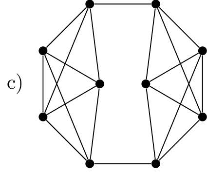
The line graph \(L(K_{3,3})\)
shown in Figure 20.2(d) has an unusual property: it
is isomorphic to its own complement.
Find one such isomorphism.
Find an \(8\)-vertex graph with
the same property.
Prove that there is no \(10\)-vertex graph with this
property.
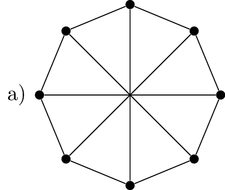
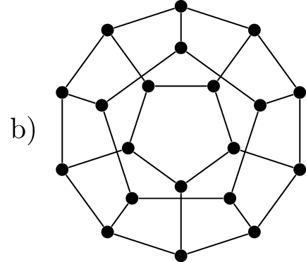
Find the edge chromatic number of the following graphs:
To complete the proof of Corollary 20.5, we need to show
that every bipartite graph \(G\) is a
subgraph of a \(\Delta(G)\)-regular
graph \(H\).
Suppose that \(G\) has a
bipartition \((A,B)\) with \(|A|=|B|\). Prove that it is possible to add
only edges to \(G\), and no new
vertices, to obtain a \(\Delta(G)\)-regular multigraph \(H\).
(How can you make use of this result if \(|A| \ne |B|\)?)
Prove that if \(\delta(G) <
\Delta(G)\), then it is possible to add edges between two copies
of \(G\) to obtain a bipartite graph
\(G'\) with \(\Delta(G') = \Delta(G)\) but \(\delta(G') = \delta(G) + 1\).
Conclude that there is a \(\Delta(G)\)-regular bipartite graph \(H\) containing \(G\) which has \(2^{\Delta(G) - \delta(G)} \cdot |V(G)|\)
vertices.
More recent proofs of Vizing’s theorem, like the one in this
chapter, are usually written so that they can also prove stronger
claims. Here are two such claims.
Modify the proof to show that if the vertices in \(G\) which have degree \(\Delta(G)\) form an independent set, then
\(\chi'(G) = \Delta(G)\).
Modify the proof to show that if the subgraph of \(G\) induced by the vertices of degree \(\Delta(G)\) is a forest, then \(\chi'(G) = \Delta(G)\).
(BMO 1992) The edges of a connected \(n\)-vertex graph \(G\) are colored red, blue, and yellow so
that each vertex has one incident edge of each color.3
Prove that \(n\) must be even
and that for all even \(n>2\), a
graph with such an edge coloring exists.
Suppose that for some subset \(S
\subseteq V(G)\), there are \(r\) red, \(b\) blue, and \(y\) yellow edges with exactly one endpoint
in \(S\). Prove that \(r,b,y\) are either all even or all
odd.
Footnotes
Don’t get stuck in an infinite loop, though. Eventually,
stop reading the sequence and go back to reading about graph theory.↩︎
As in Chapter 19, this is really the
definition of a proper edge coloring, but we will not consider
any other kind.↩︎
I have paraphrased; the original problem on the British
Mathematical Olympiad had an elaborate and very long statement about
dwarfs and orcs.↩︎