Before you begin learning about specific problems in graph theory, I
want to convince you that graph theory is useful. Well, of course I
would say that—I’m a graph theorist! However, one of the reasons I’m
firmly convinced that graph theory is one of the most highly applicable
areas of math is that I often find it fruitful to think about the world
graph-theoretically even when I’m not trying to solve problems in graph
theory.
This comes easier to me, because I’ve spent many years with all this
graph-theoretic language at my fingertips. It will not come easily to
you at first, when you don’t know any graph theory. So one of them
things I want to do here is to show you how I think about turning a
problem into a graph. Stop and think about it yourself! Think about it
with each new example.
I want to limit myself to examples that are simple enough to fully
explain in this chapter. However, I also want to give complete examples
that I can fully describe to you. Finally, I want to give you a variety
of examples: I want to show you different types of problems in graph
theory, and I want to show you very different flavors of applications,
as well.
I will ask many questions about the graphs in this chapter, and I
will often give formal mathematical names for the answers to those
questions. However, I will not answer the questions here, and you should
not feel obligated to learn any of the fancy terminology yet: the only
terms I am asking you to learn at this point are those set aside in a
“Definition 1.x” paragraph. If you become curious about
the other ideas mentioned here—good! However, you will have to wait
until a later chapter.
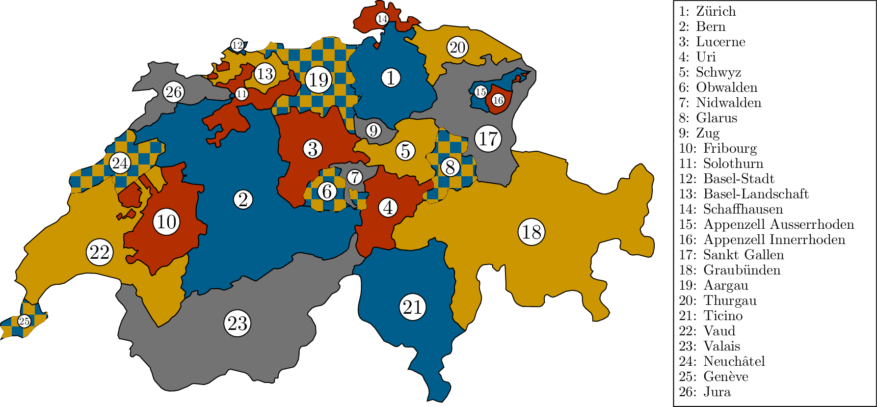
Switzerland (formally known as the Swiss Confederation) is made up of
\(26\) cantons. On a map, you will
often see these drawn in different colors, to make the borders between
different cantons clearer to see. As a result, it’s particularly
important to choose the colors for each canton so that adjacent cantons
receive different colors.
I have used five different colors to color the map in Figure 1.1. This is a bit unfortunate,
because the color palette I’ve picked out to use throughout this book
contains only four colors. Several of the cantons are given a
checkerboard pattern instead of a solid color, which makes it somewhat
harder to see where the borders lie.
Could we color the map of Switzerland with four colors?1 And
what is the minimum number of colors needed? The answer to that question
is called the chromatic number of the graph that describes the
problem—but to say that properly, we first have to say what a graph
is.
This is not the same “graph” that you would encounter in high school
algebra! Blame the Greeks: in Greek, the root “graph” just means
“picture”, and there are quite a few things in mathematics that we want
to draw pictures of, so there is some overlap in terminology as
well.
Unfortunately, the word is particularly awkward in the context of
graph theory, because here the graphs are specifically not pictures!
Instead, a graph is going to be exactly the mathematical object that we
need to ask questions like, “How many colors are necessary to color the
cantons of Switzerland?” Before giving the definition, it’s worth
thinking about the things we do and don’t need to know:
We don’t need to know that the canton of Thurgau is in the north
part of eastern Switzerland, nor that it’s shaped roughly like a shark
(in my opinion).
We also don’t need to know that it’s called “Thurgau”, as opposed
to “Thurgovia” (its anglicized name) or “\(20\)” (the numerical label it is given in
Figure 1.1) or anything else. We will
need to refer to the cantons individually somehow, or else it would be
very hard to talk about which cantons get which colors. However, it doesn’t
matter at all which names we give them.
We do need to know that Thurgau (or 20, or whatever we choose to
call it) borders Schaffhausen (14), Sankt Gallen (17), and Zürich (1):
if we want to color the map so that adjacent cantons get different
colors, then these are the colors we’ll need to distinguish.
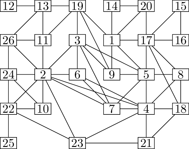
Two schematic representations of the Switzerland
graph
For example, consider the diagrams in Figure 1.2, in which the cantons
have been replaced by short numerical labels or even just plain dots,
and their placement only loosely reflects their geographic location.
This is just as good for our purposes; maybe even better, because it
does not include any distracting details!
Even having a diagram at all is a concession to our human needs. If
we wanted to try to use a computer to solve the problem, we might simply
enter the following (which, under the hood, is how the two diagrams in
Figure 1.2 were generated):
With that in mind, let us finally give the definition of a graph,
which will reflect all of these thoughts and only keep what is truly
important. This definition can be used in many ways, to capture all
kinds of relationships between all kinds of objects; I hope that the
examples in this chapter give you an intuitive understanding of how to
use it.
Definition 1.1. A graph\(G\) is a pair \((V,E)\) where:
\(V\) is a set of arbitrary
objects called vertices; a single one is called a
vertex. In the Switzerland graph, \(V\) is the set of the \(26\) cantons. We write \(V(G)\) for the set of vertices of a graph
\(G\).
\(E\) is a set of
edges: each edge is an unordered pair of vertices, or
just a set of two vertices. In the Switzerland graph, \(E\) is the set of all pairs of cantons that
share a border. We write \(E(G)\) for
the set of edges of a graph \(G\).
Since an edge is a set of two vertices, it should be written with the
notation \(\{x,y\}\), but to avoid too
many symbols in notation that is used all the time, graph theorists
often skip the curly brackets and just write \(xy\). I will do the same in this book, only
using set notation when it’s necessary to avoid ambiguity. For example,
we should not represent an edge in the Switzerland graph as “\(117\)”, because it’s not clear if this
means \(\{1,17\}\) or \(\{11,7\}\).
There is a lot of secondary terminology to describe the relationship
between edges and vertices in a graph. Here are a few of the most
important terms:
Definition 1.2. Vertices \(x\) and \(y\) in a graph \(G\) are adjacent when
\(G\) has an edge \(xy\); we also say that \(x\) is a neighbor of \(y\) (and vice versa).
Definition 1.3. The endpoints
of the edge \(xy\) are the vertices
\(x\) and \(y\). An edge is incident
to its endpoints, and vice versa: \(x\)
and \(y\) are incident to \(xy\), and \(xy\) is incident to \(x\) and \(y\).
It’s also okay to say that an edge \(xy\) goes between \(x\) and \(y\), or joins \(x\) and \(y\), for example; these are not really
technical terms, but just English words used in the ordinary way to
convey relationships in a graph. As long as it’s clear what you mean,
the exact words you use are flexible. Avoid using words like “connect”
or “connected” informally, though: they have a technical meaning in
graph theory.
In Chapter 19 we will define a
coloring of a graph \(G\) to
be a function from \(V(G)\) to some
set \(C\) whose elements we will call
“colors”. An actual non-mathematical coloring of a map, such as in
Figure 1.1, can be described by such a
function: for example, \(f(20)=\text{blue}\) might describe coloring
Thurgau blue. In this model of coloring, we will see how to prove lower
and upper bounds on the number of colors needed.
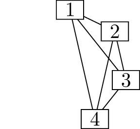
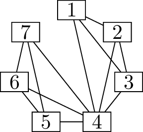
The seven dwarfs
One day, the seven dwarfs of fairytale2
wanted to play cards. Unfortunately, they only have one deck of cards.
Their favorite card game, Hearts, is a four-player game, so only four
dwarfs can play at a time. If the dwarfs switch in and out of the game,
how many rounds will they need to play so that every dwarf has gone up
against every other dwarf at least once?
It seems reasonable to start with two games that don’t overlap very
much: for example, a game with dwarfs 1–4 followed by a
game with dwarfs 4–7. After that, though, we might need some help
keeping track of which dwarf has already played which other dwarf. Since
this is a property of different pairs of dwarfs, it is natural to model
it with a graph whose vertices are the dwarfs. Figure 1.3(a) shows the pairs of dwarfs that
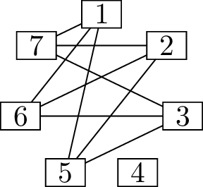
face each other in the first game; Figure 1.3(b) shows
the status after both games; finally, Figure 1.3(c) shows the pairs of dwarfs
that have yet to face each other.
The first card gameThe first two gamesThe missing matchups
The seven dwarfs
I admit that I chose this example with an ulterior motive: to
illustrate a few common operations on graphs. Graphs are built out of
sets, and the fundamental operations of set theory—union, intersection,
and complement—all show up graph theory, as well.
The graph in Figure 1.3(b) is
assembled out of two graphs: the graph in Figure 1.3(a) which tracks only the first
card game, and a similar graph (not pictured) which tracks only the
second card game. This is the operation we’ll define to be the union of
two graphs.
Definition 1.4. The union\(G \cup H\) of two graphs \(G\) and \(H\) is the graph with all vertices and
edges appearing in at least one of the two graphs: \(V(G \cup H) = V(G) \cup V(H)\) and \(E(G \cup H) = E(G) \cup E(H)\).
The union \(G \cup H\) is called
a disjoint union if \(G\) and \(H\) share no vertices or edges.
No; even though the graphs of the two card
games share no edges, vertex 4 appears in both graphs.
We could also define the graph intersection \(G \cap H\) to be the graph that only keeps
the vertices and edges common between \(G\) and \(H\), but that is a much less common
operation.
Finally, we get to the complement. This is an awkward operation to
define in set theory. If \(\overline
S\) is the set of all objects not appearing in \(S\), then we can probably all agree that a
complement like \(\overline{\{1,2\}}\)
contains the element \(3\), but does it
contain the element \(\pi\)? What about
the color purple? So in serious set theory, it’s much more common to use
the relative complement, or set difference, \(A-B\): the set of all objects appearing in
\(A\), but not \(B\). We will see plenty of set differences
in this book too, but fortunately, there is a natural notion of
complement when it comes to graphs.
The graphs have the same \(7\) vertices, but the graph in Figure 1.3(c) has exactly the edges that
Figure 1.3(b) does not have.
This is the definition we make in general:
Definition 1.5. The complement\(\overline G\) of a graph \(G\) is the graph with \(V(\overline G) = V(G)\) such that two
vertices \(x\) and \(y\) are adjacent in \(\overline G\) exactly when they are not
adjacent in \(G\).
It would be unkind of us to use the dwarfs as an example of unions
and complements without addressing their concerns about how to schedule
their card games. Graphs can help with that as well. We can get a
preliminary answer just by counting edges.
How many pairs of dwarfs are there, and
how many face each other in each game? What does this tell us?
Altogether, there are \(\binom 72 = \frac{7\cdot 6}{2} = 21\)
pairs3 of dwarfs: we choose two dwarfs in
\(7\cdot 6\) ways, and divide by \(2\) because order doesn’t matter. In each
card game, \(\binom 42 = 6\) dwarfs
face each other, so at least \(21/6\)
games are necessary, which rounds up to \(4\).
Unfortunately, if the dwarfs play two games as in Figure 1.3, they can’t finish by playing
two more. A single card game can only take care of \(4\) of the \(12\) remaining edges in Figure 1.3(c), so at leas three more
card games are needed. (See if you can find \(3\) card games that will do it!) We can’t
avoid arriving at the graph in Figure 1.3(c)
entirely, either! It occurs whenever there are two card games that only
have one dwarf in common. But if this never happens, then every dwarf
needs at least three games to face all \(6\) other dwarfs, and this leads to an even
longer solution. Ultimately, at least five card games are necessary,
however we schedule them.
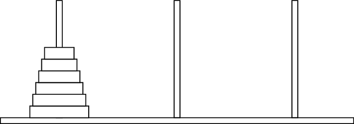
The Towers of Hanoi
The Towers of Hanoi puzzle was invented in 1883 by Édouard
Lucas [6]; it is now so
popular its origins have been nearly forgotten. In this puzzle, you have
three pegs, and some number of disks of different sizes stacked on the
pegs. Initially, all the disks are placed on one peg, sorted by size
(with the smallest disk on top), as shown in Figure 1.4.
The Towers of Hanoi puzzle
You are allowed to move the disks in a limited way: in a single move,
you can lift the top disk on a peg, and put it down on another peg,
provided you do not place a larger disk on top of a smaller one. Placing
a larger disk on a smaller one is always forbidden. The goal of the
puzzle is to move all the disks from one peg to another.
How can we model this puzzle as a graph? This is a much trickier
question than in the previous section, and the answer may be
counter-intuitive the first time you see something like it. When I’ve
asked the question to clever students new to graph theory, they’ve been
tempted to start with either the disks or the pegs as the vertices,
which turns out not to lead us anywhere fruitful.
To arrive at a useful answer, I suggest thinking as follows: how can
we define a graph that will know everything about the rules of this
puzzle, so that when we try to use graph theory to solve it, we will not
need to know anything? Our graph does not need to be a small, efficient
representation of the rules, either. On the contrary: if the solution to
the puzzle (which may be a very long sequence of moves) is to be found
anywhere in the graph, then the graph will have to be pretty big.
The strategy we take to model the Towers of Hanoi puzzle as a graph
\(G\) is to do the following:
Let the vertex set \(V(G)\) be
the set of all possible states of the puzzle. For example, the picture
in Figure 1.4 is just one of the
vertices. If we take the smallest disk and move it to the middle peg,
the result is a different state of the puzzle, represented by another
vertex. Our final goal is to have all the disks stacked up on a
different peg, which is yet another vertex.
Let the edge set \(E(G)\) be the
set of all possible pairs \(xy\) where
it’s possible to turn state \(x\) into
state \(y\) by making a single move.
Or, phrased more concisely: let two states \(x,y \in V(G)\) be adjacent if a single move
can turn \(x\) into \(y\).
(This is a symmetric relationship: if we can move a disk from one peg
to another, we can always move it back.)
In a graph, our edges should be unordered
pairs, but the rule “a single move can turn \(x\) into \(y\)” seems like an ordered relationship. Is
this a problem?
Not in this case, because if we can move a
disk from one peg to another, we can always move it back, so the
relationship is symmetric. Puzzles where we cannot always reverse a move
we make are more difficult to model.
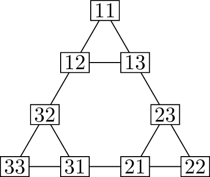
The graph representing a \(2\)-disk Towers of Hanoi
puzzle
As you might imagine, this definition of \(V(G)\) results in a large graph \(G\) indeed. So in Figure 1.5, the graph \(G\) is illustrated for a version of the
puzzle with only \(2\) disks: a small
one and a large one. The two-digit label on each vertex records the
positions of the two disks: the first digit records the position of the
bigger disk, and the second digit records the position of the smaller
disk. In this way, the two-digit number describes the state of the
two-disk Towers of Hanoi puzzle. (In our definition, we said that \(V(G)\) is the set of all possible states of
the puzzle, but we didn’t specify how the states of the puzzle are
encoded. That’s because it doesn’t really matter!)
In Figure 1.5, which vertices
represent our starting state and our final state?
The vertices \(11\), \(22\), and \(33\) are the three vertices in which both
disks are stacked on the same peg; we want to get from one of these to
another.
What do the edges from vertex \(12\) to vertices \(11\), \(13\), and \(32\) represent?
The smaller disk can be moved from peg
\(2\) to peg \(1\) or peg \(3\); these moves give us the edges from
\(12\) to \(11\) and \(13\). The bigger disk can only be moved
from peg \(1\) to peg \(3\), giving the edge from \(12\) to \(32\); it cannot be moved to peg \(2\), because it cannot be placed on top of
the smaller disk.
Now that we have the graph, how do we think about solving the puzzle?
To answer that question, let’s think about what happens in the world of
graph theory when we attempt to solve the puzzle by moving disks around.
Each time we lift a disk and move it to a different peg, we go from one
state of the puzzle to another: from one vertex to another. Suppose we
make \(m\) moves; then we can imagine
recording the entire history of the moves we’ve made as a sequence \[(x_0, x_1, x_2, \dots, x_{m-1}, x_m)\] in
which each term \(x_i\) is a vertex in
the Towers of Hanoi graph. The moves that we’ve made are valid moves if
it’s the case that for all \(i=1, \dots,
m\), the pair \(x_{i-1} x_i\) is
an edge of the Towers of Hanoi graph.
In graph-theoretic terminology, such a sequence is called a
walk from \(x_0\) to \(x_m\), or an “\(x_0 - x_m\) walk” for short; see Chapter 3 for more details. When we’re
talking about puzzles like the Towers of Hanoi, that’s a very
metaphorical walk: you could picture a little figure standing on the
diagram in Figure 1.5 and walking along the
edges, but that figure exists only in your imagination. It would become
a much more literal walk in the Switzerland graph from the previous
section! Suppose that you live in Zürich, and you decide to go on a hike
through Switzerland until you reach Geneva. Then the sequence of cantons
you walk through (updated every time you cross a border between cantons)
will be a walk in the Switzerland graph: a \(1-25\) walk where \(1\) is the Canton of Zürich and \(25\) is the Canton of Geneva.
A solution to the Towers of Hanoi puzzle is a walk with very specific
starting and ending vertices: we want to start in a vertex \(x_0\) corresponding to all disks being on a
single peg, and we want to end in a vertex \(x_m\) corresponding to all disks being on
some other single peg. The length of this walk, \(m\), is the number of moves that we needed
to make, so our second goal might be to minimize this length and find
the shortest solution.
The question of finding minimum-length walks in a graph is not only
useful for puzzles. If you were to ask your phone for walking directions
from Zürich to Geneva, it would consult a much bigger graph: the graph
of possible pedestrian locations in Switzerland, at a fairly low
resolution, and with additional metadata such as walking times that
we’re not considering yet. However, in that bigger graph, it would solve
essentially the same problem of finding a minimum-length walk!
A tiling puzzle
Here is a different kind of puzzle. (I promise that graph theory is
not just good for puzzles! However, puzzles are a very convenient
application: they usually have much simpler rules than the real world,
so we can describe them cleanly using graph theory, and puzzle creators
often at least try to make their puzzles fun.)
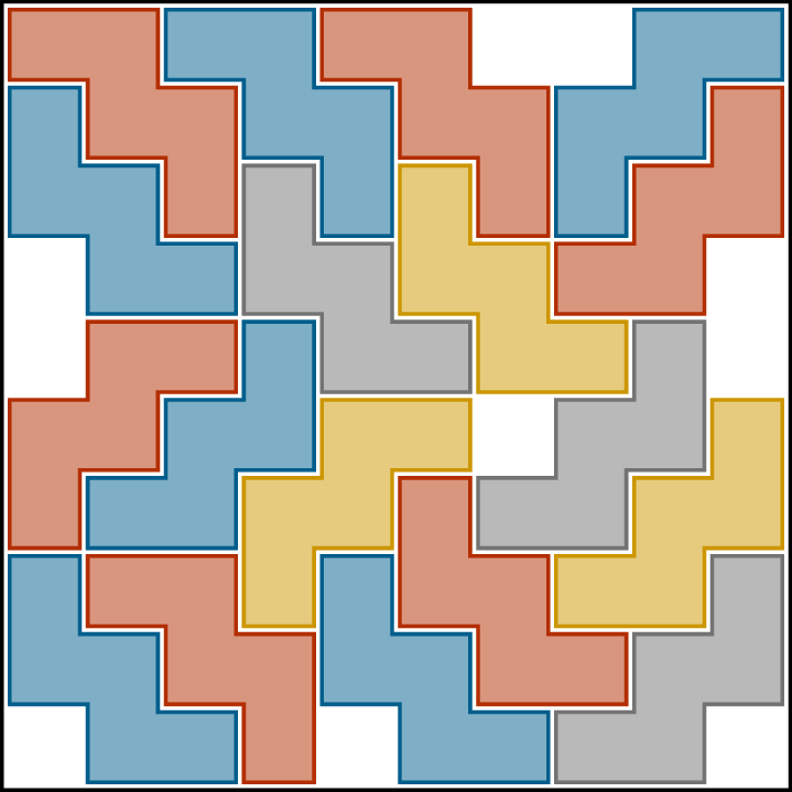
Suppose that you have an infinite supply of zigzag-shaped tiles made up of five \(1\times 1\) squares. How many of
them can you place on a \(10 \times
10\) grid without overlap? One possible optimal solution to this
problem is shown in Figure 1.6.
A solution to fitting \(18\) zigzag tiles in a \(10\times 10\) grid without
overlap
How did I find this solution? I did it by encoding the problem as a
graph and using some tools in Mathematica’s graph theory library. It’s
not obvious how to represent this as a graph theory problem, but here is
what I ended up doing:
Let the vertices be all ways to place a single tile on the \(10 \times 10\) grid.
Put an edge between two vertices if the tile placements they
represent are incompatible: the tiles would overlap.
How many vertices does this graph
have?
The middle square of a tile can be in any
of the \(8^2 = 64\) squares that are
not on the edges of the \(10\times 10\)
grid. Once we pick where the middle square goes, there are \(4\) ways to orient the tile, for a total of
\(64 \cdot 4 = 256\) placements.
A solution to the puzzle is a collection of locations where we’ve
placed tiles, so it’s a set of vertices in this graph.
Which sets of vertices are valid solutions
to the puzzle?
A set of vertices tells us where to place
tiles, but it’s only a valid solution if none of the tiles we place
overlap. Overlapping tiles are represented by edges, so we want a set in
which no two vertices are adjacent.
A set of vertices with no edges between them is called an
independent set in a graph, and we will look at the problem of
finding these in Chapter 18.
In fact, there is a second way to think about the problem that’s
equally good. We could have defined two vertices to be adjacent if the
tiles would not overlap: this graph would be the complement of the graph
we originally defined. In the complement graph, a conflict-free solution
corresponds to a clique: a set of vertices in which any two
vertices are adjacent. Cliques and independent sets are both important;
though the problems they solve are equivalent, as we see here, sometimes
one is more natural than the other to think about, and sometimes we
study the relationship between the two problems.
Finding the largest independent set in a \(256\)-vertex graph is a lot for a human,
but not out of the reach of computer algorithms. It took my laptop \(48\) seconds to find the largest
independent set in the graph: less time than it took me to describe the
problem to my computer!
Taking photos efficiently
Here is an application of graph theory to engineering.4
Suppose you want to inspect a manufactured part for quality by first
taking photos of it from many different angles. You don’t have to do
this yourself: you have a many-jointed robot arm with a camera at the
end, and the robot arm can move around to take the pictures for you. How
can you program the robot arm to take the photos as efficiently as
possible?
Just as in the Towers of Hanoi puzzle, we can describe this problem
in terms of walks through a graph, though the setup and our goals are
both different. This leads us to a good model of the problem with graph
theory: if we want the robot arm’s trajectory to be a sequence of
vertices in a graph, then each vertex should be a position the robot arm
can be in. We may as well limit the vertices to just the positions in
which we want the robot arm to take a photo—those are the interesting
ones.
Why not take our vertex set to be the set
of all positions the robot arm can be in?
The only reason not to is that there might
be too many of these. In fact, if you imagine the robot arm moving
continuously, there might be infinitely many vertices, which is
definitely too many!
Just as in the Towers of Hanoi graph, we want our edges to represent
ways that the robot arm can move. However, in principle, from any
position, the robot arm can twist itself around to move to any other
position. There might not be a good notion of “elementary” motions: we
might even end up making all pairs of vertices adjacent.
Which relevant piece of information is
missing from such a model?
The time that it takes for the robot arm
to move from one position to another.
In such an application, it makes sense to consider a weighted
graph (discussed in more detail in Chapter 9). Each edge
in the graph represents a movement of the robot arm from one state to
another, and it may well be that every pair of states has an edge
between them. However, some motions take more time than others, so each
of our edges has a nonnegative real number linked to it: the time to
complete that motion. That’s what a weighted graph is: each edge has a
number on it that we call its weight, or perhaps its
cost.
The example of the robot arm is only one instance of this problem
appearing in applications: there are many situations that can be modeled
by visiting all the vertices of a graph as efficiently as possible!
If we have a walk in a weighted graph,
what quantity measures how good it is?
Instead of the length of the walk, we
measure its total cost (or total weight): the sum of the weights of the
edges. In our application, that’s the time it takes the robot to visit
all the photo-taking positions and take all the photos.
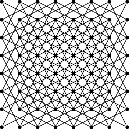
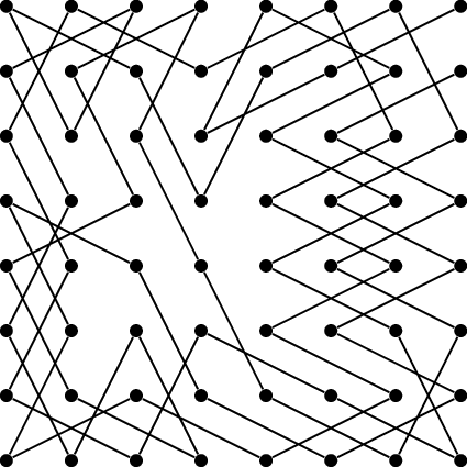
The \(8\times 8\) knight
graphA Hamilton path in the graph
The knight’s tour problem
An ordinary graph can be thought of as a weighted graph in which
every edge has the same weight, which might as well be \(1\). (We can also pretend that every edge
the graph doesn’t have is present with a weight of \(\infty\), so that we really really don’t
want to use it in an efficient solution.) In this case, a perfect
solution to the problem would be a walk through the graph that visits
every vertex exactly once: if there are \(n\) vertices, the walk takes \(n-1\) edges, which is the least number
possible. In such a case, the graph has a Hamilton path: these
are discussed in Chapter 17
of this book.
Here is another example of two very different problems becoming the
same when considered from the point of view of graph theory. In chess,
the “knight’s tour” problem is to move a knight around the chessboard
and visit each square exactly once. The graph we consider for this
problem is the \(8\times 8\) knight
graph, shown in Figure 1.7(a): the graph with a
vertex for every square of the chessboard, and edges representing the
valid knight moves. A Hamilton path in this graph, shown in Figure 1.7(b), is precisely a knight’s
tour of the chessboard.
Match the cars and drivers
A final flavor of puzzle that is secretly all about graph theory is
the “logic grid puzzle”, or “matching puzzle”. Here is a beginner-level
example.
Five friends named Rod, Sal, Teresa, Victor, and Whitney own cars in
five different colors: white, blue, black, red, and green. The following
three things are known about the colors of their cars:
Neither Victor nor Teresa own a car in a color that appears on
the United States flag (red, white, or blue).
Even though the sounds of their names would suggest it, Rod’s car
is not red and Whitney’s car is not white.
Rod and Victor like bright colors, and would not drive a black or
white car.
Given this information, can you identify the color of the car each of
them drives?
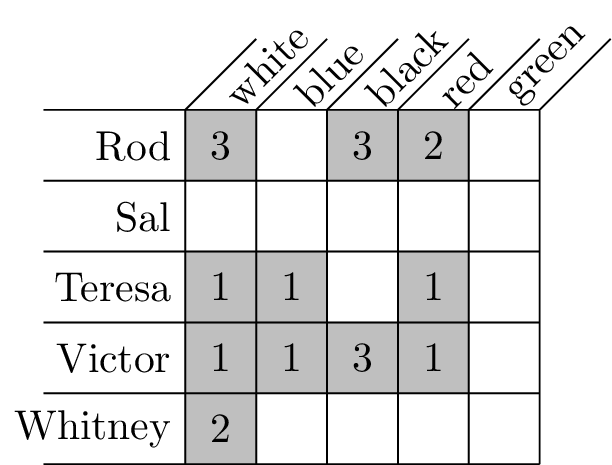
The classic way to solve a puzzle like this is to draw a grid to
represent the data; in this case, the rows would be the \(5\) people in the problem, and the columns
would be the \(5\) colors. Then, the
cells of the grid representing impossible combinations are shaded in to
eliminate them: in Figure 1.8(a), this
is shown with a number in each shaded cell indicating the statement that
lets us eliminate it. From there, we can try to make deductions and use
them to eliminate more cells. I have given you an example that has a
unique solution, so you can try solving it, if you like.
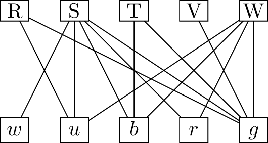
Logic grid representing the puzzleBipartite graph representing the puzzle
Two ways to think about matching cars to people
Figure 1.8(b) shows another way to
think about the logic puzzle: as a graph. In this graph,
The vertices come in two types: five vertices representing the
people (labeled R, S, T, V, W in the diagram) and five vertices
representing the colors (labeled \(w\),
\(u\), \(b\), \(r\), \(g\)
in the diagram).
There is an edge from each person to each car the three
conditions permit them to drive.
This graph is called a bipartite graph because its vertices
can be split into two non-overlapping sets such that all edges have one
endpoint in each set. In this case, the two sets are the people and the
cars. The solution to the puzzle is a perfect matching in the
graph: a set of edges that have each of the vertices as an endpoint
exactly once. Both of these concepts will be introduced in detail in
Chapter 13.
How many edges does a perfect matching
contain?
In this problem, it will be \(5\) edges. In general, if our graph has
\(n\) vertices, a perfect matching
should have \(n/2\) edges, because each
of the edges has \(2\) endpoints,
covering \(2\) of the \(n\) vertices.
Figure 1.8(b) is not necessarily
the best visualization if you want to try to solve the logic puzzle.
However, thinking about the problem as a graph is rewarding for two
reasons:
We can make connections to other problems that look superfically
different in how they’re phrased, but turn out to be the same problem in
the language of graph theory.
Perfect matchings are not just for logic grid puzzles! On a college
campus, they can be used for matching together instructors with classes,
or interns with internships, or roommates in college dorms. They are
also a common subroutine for more complicated optimization
problems.
There are general graph-theoretic guarantees that apply to all
these applications equally well. Later on in this book, we will see what
conditions guarantee the existence of a perfect matching, and even
investigate whether the solution is unique.
Suppose a graph has \(n=99\) vertices. Then a perfect matching
should have \(n/2\) edges, which is
\(49.5\). How can we make sense of
this?
In a graph with \(99\) vertices (or any other odd number), a
perfect matching cannot exist—so it’s okay that our formula gives a
nonsense answer. If we have \(99\)
objects, we cannot divide them into pairs; one object will be left out
at the end.
Practice problems
Describe how to use a graph to model each of the following
puzzles:
A word ladder puzzle, in which one word must be transformed into
another by changing one letter at a time. For example, if the goal were
to get from “graph” to “Euler”, one possible solution might be: \[\text{graph} \to \text{grape} \to \text{grade}
\to \text{grads} \to
\text{goads} \to \text{golds} \to\]\[\to \text{bolds} \to \text{boles} \to
\text{roles} \to \text{rules} \to \text{ruler} \to
\text{Euler}.\]
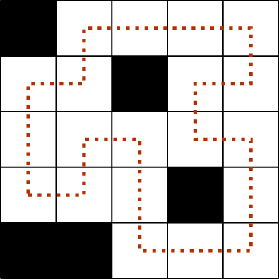
A pure loop puzzle, in which several squares of an \(n\times n\) grid are shaded, and the goal
is to draw a closed loop through the unshaded squares that visits each
of them exactly once. Such a puzzle and its solution are shown in the
first diagram below.
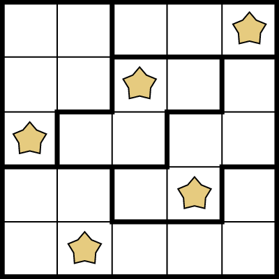
A star battle puzzle, in which an \(n\times n\) grid is divided into several
regions, and a star must be placed in each region so that no two stars
occupy the same row or column, and no two stars are adjacent even
diagonally. Such a puzzle and its solution are shown in the second
diagram above.
The country of Hungary is divided into \(7\) regions, which are further subdivided
into \(19\) counties (and the capital,
Budapest, which is not part of any county). Look these up on a map of
Hungary; then, draw a graph diagram, similar to one of the diagrams in
Figure 1.2,
of the \(7\) regions, if you
just want a bit of practice, or
of the \(19\) counties and
Budapest, if you want to draw a bigger graph.
Briefly explain (without checking any cases by brute force) why
the cantons of Switzerland cannot be colored with just three colors so
that no two adjacent cantons have the same color.
To study the graph representing a \(3\)-disk Towers of Hanoi puzzle, we might
label the states by \(3\)-digit
sequences \(111\) through \(333\); each digit represents the location
of a disk, from largest to smallest.
For this problem, let \(H_n\) denote
the \(n\)-disk Towers of Hanoi graph;
Figure 1.5 is a diagram of \(H_2\).
Draw only one part of \(H_3\):
the part containing the \(9\) vertices
111, 112, 113, 121, 122, 123, 131, 132, and 133.
Extrapolate from what you’ve done to draw all of \(H_3\).
How many vertices does \(H_n\)
have, as a function of \(n\)?
How many edges does \(H_2\)
have? What about \(H_3\)? What about
\(H_n\), as a function of \(n\)?
The zigzag tile graph from this chapter is too large for you to
draw by hand, so let’s look at a much simpler problem of the same
type.
Suppose we are trying to place \(2 \times
2\) square tiles on a \(4 \times
4\) grid without overlap.
Draw a diagram of the graph where the vertices are ways to place
a single \(2\times 2\) tile on the grid
(there should be \(9\) vertices), with
an edge between two vertices when the tile placements they represent are
incompatible.
Find an independent set in the graph representing the “boring”
solution, which places four \(2\times
2\) square tiles covering the entire grid.
Find some other interesting non-overlapping tile placement in the
grid, and find the independent set in your graph that corresponds to
it.
This is more of a puzzle than a graph-theoretical question: find
a way to fit \(12\) zigzag-shaped tiles
into an \(8\times 8\) grid with no
overlaps. (How do we know that this is optimal without the use of a
computer program?)
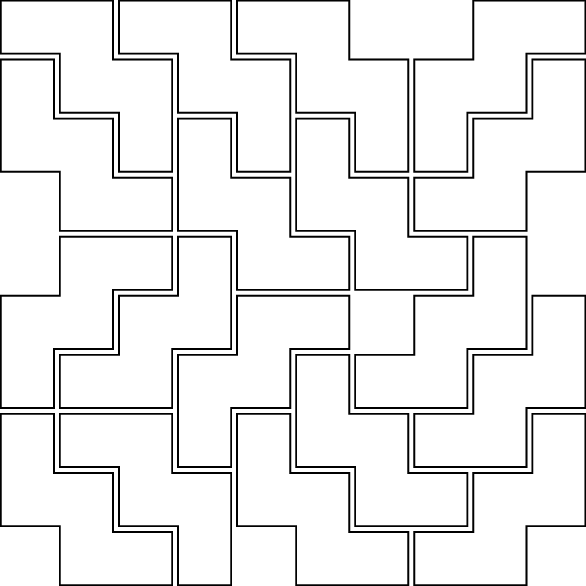
Find a way to color the tiling below using only 3 colors so that
no two tiles that share a border have the same color.
A knight in chess moves by jumping to another square two steps in
one direction and one step in a perpendicular direction. (Some knight
moves are illustrated in Figure 1.7.)
Find a knight’s tour of the \(5 \times
5\) chessboard, shown below.
Prove that all such tours must begin and end on a dark-colored
square.
Footnotes
If you already know a bit of the relevant theory, and
think that you’ve heard of a powerful result that solves this problem:
Switzerland has a bit of a surprise for you! The full solution takes a
bit more work.↩︎
To avoid any potential entanglements with Disney, I will
use the traditional names for the seven dwarfs: Dwarf 1 through
Dwarf 7.↩︎
If you haven’t seen binomial coefficients \(\binom nk\) yet in your mathematical
career, the only one you’ll need to know for \(99\%\) of graph theory is \(\binom n2 = \frac{n(n-1)}{2}\): this counts
the number of unordered pairs of \(n\)
objects, or the number of possible edges an \(n\)-vertex graph could have.↩︎
I found it in a 2022 paper by Bottin, Boschetti, and
Rosati [10], but I am
not an expert in robotics, so I don’t know enough to put that paper in
the context of its field—I just thought it was cool.↩︎