Graph coloring is one of the iconic problems in graph theory, though
usually people think of it in the context of coloring maps. This
application was mentioned in Chapter 1, and we will see it in
detail later, in Chapter 24. The
applications you will see in this chapter are more metaphorical versions
of coloring—but that’s par for the course in graph theory, which is all
about representing the world with metaphorical points and metaphorical
lines.
I begin this chapter with one upper bound and two lower bounds on
chromatic number, and I think these are the basics you should know of
the theory of graph coloring. Meanwhile, Theorem 19.4 and Theorem 19.7 demonstrate how these basics can
be used. The motivation for these specific demonstrations is to show you
an example where the clique bound of Proposition 19.2 is very useful, and
an example where it’s not at all useful; in either case, I hope that it
gives you a sense of why the clique number does not necessarily tell us
the chromatic number.
Brooks’ theorem (which describes the conditions under which \(\chi(G) \le \Delta(G)\)) is a common result
to cover in an introductory graph theory class, but I’ve left it out. I
have done this because I think seeing it for the first time at this
point is extraordinarily uncompelling—and I say this as someone who has
both used the theorem in research and taught a week-long class about
variants of the theorem. When you just start out learning about graph
coloring, it is unsatisfying to go to great effort to improve
Proposition 19.1 by a tiny amount. I
recommend seeing Brooks’ theorem for the first time as a more
experienced graph theorist, for example by reading “Brooks’ Theorem and
Beyond” by Cranston and Rabern [21], which presents a variety of proofs of
the theorem and its extensions.
Graph coloring and Sudoku
A Sudoku puzzleThe \(4\times 4\) Sudoku
graph
Sudoku puzzles and graph coloring
In case you have never encountered a Sudoku puzzle, let me explain
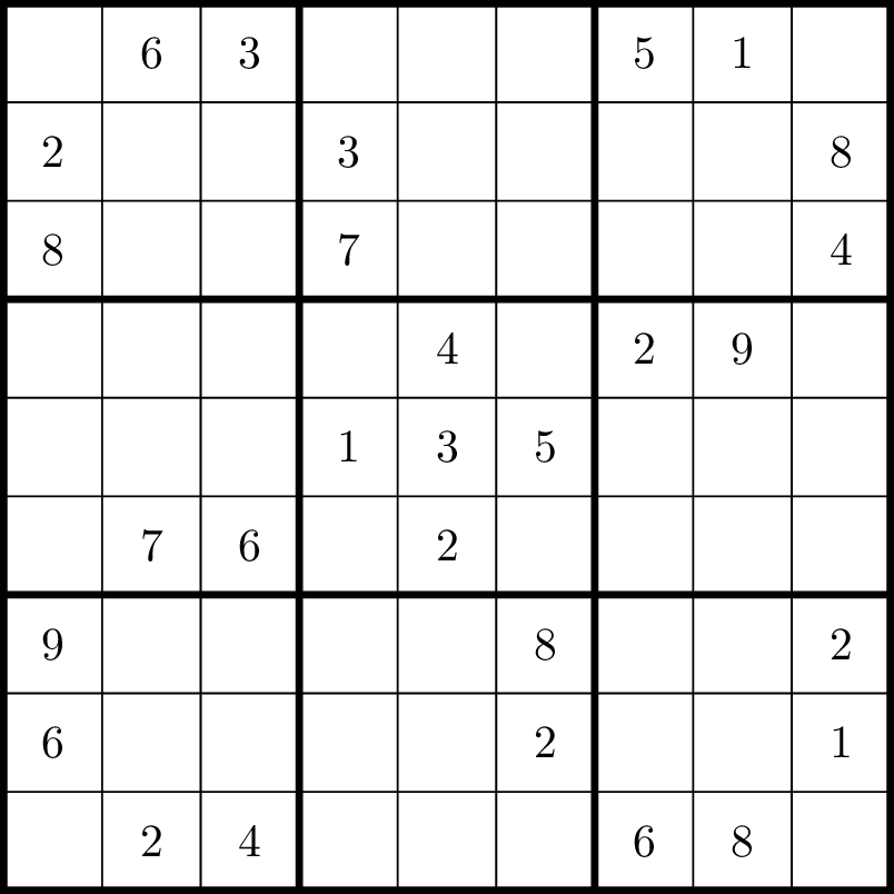
how they work. Figure 19.1(a)
shows an example of a Sudoku puzzle. It is a \(9 \times 9\) grid, with its \(81\) cells grouped together into \(9\) boxes. Some of the cells already have
numbers in them. The objective of the puzzle is to figure out which
numbers should go in the empty cells! The rule is that in each row, each
column, and each \(3\times 3\) box, the
nine cells should contain the numbers 1 through 9 in some order.
For example, the top left corner of Figure 19.1(a) could not contain the numbers
\(2, 3, 6, 8\), because they are
already present in its \(3\times 3\)
box; it could also not contain the numbers \(1, 5\) (already present in its row) or
\(9\) (already present in its column).
The numbers \(4\) or \(7\) have not been ruled out, though only
one of them is correct; the other would eventually lead to a
contradiction if you wrote it in, even though there’s no obvious problem
yet.
As usual, we would like to turn this logic puzzle into a problem of
graph theory. The first task is to choose a graph to model it with.
Although other options exist, for us it will be most convenient to make
the \(81\) cells in the grid be the
vertices of the Sudoku graph. Make two cells adjacent in this graph if
they are in the same row, the same column, or the same \(3 \times 3\) box.
How can the rules of Sudoku be expressed
in terms of the edges of this graph?
The goal of Sudoku is now to assign one of
the numbers 1 through 9 to each vertex of the graph, so that adjacent
vertices are assigned different numbers.
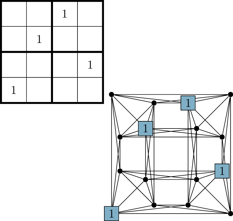
Since a diagram of this Sudoku graph would look like utter chaos and
not give you any intuition at all, I have drawn a diagram of the \(4\times 4\) Sudoku graph in Figure 19.1(b). In \(4\times 4\) Sudoku, the rules are the same,
except that each row, column, and \(2\times
2\) box has four numbers in it, and the cells are allowed to
contain the numbers 1 through 4.
In Figure 19.1(b), the
1’s are all entered into the grid (and shown in the graph). In general,
what can you say about the set of all vertices assigned the number \(1\) in a Sudoku puzzle?
Two adjacent vertices cannot both be
assigned the number \(1\), so the set
of vertices with a \(1\) must be an
independent set.
The graph-theoretic rules of Sudoku happen to match a well-studied
problem in graph theory, which is why I used Sudoku as an example to
begin this chapter. For historical reasons, rather than assigning every
vertex a number, we assign every vertex a color. For practical reasons,
graph theorists are very flexible about what “colors” are. It’s fine to
say, “We will use the set of colors \(\{1,2,\dots,9\}\),” for example, in which
case the numbers in a Sudoku grid are our colors.
Definition 19.1. A proper
coloring (or just coloring) of a graph \(G\) is a function \(f\colon V(G) \to C\) such that for all
edges \(xy \in E(G)\), \(f(x) \ne f(y)\). The elements of \(C\) are called colors, but can be any set
we like.
Allow me to justify my terminology. The term “proper coloring” is the
formal name for a coloring \(f\) with
the condition that \(f(x) \ne f(y)\)
for all edges \(xy\), so that’s what we
should be using. However, almost every single time we color something in
this book, we will want a proper coloring. To omit needless words, I
will simply say “coloring” unless emphasis is needed: for example, when
we want to check that a coloring \(f\)
really is proper. On the rare occasion where we want a coloring that
might give the same color to both endpoints of an edge, I will call it
an improper coloring to emphasize this.
Back to graph theory! Sometimes it is convenient to think about
coloring a graph in a different way: not as a function, but as a
partition. We say that a color class of a coloring is a
set of of all vertices of some color. Every vertex is in exactly one
color class, so the color classes are a partition of \(V(G)\); a coloring is proper if and only if
the endpoints of every edge are in different color classes.
What are the color classes in the solution
to a Sudoku puzzle?
There are \(9\) of them: for each number from \(1\) to \(9\), the set of all cells containing that
number is a color class.
The study of graph coloring originated with a very practical coloring
problem: given a map divided into several regions, how can we color the
regions so that neighboring regions receive different colors? This is a
coloring of the graph of adjacencies of the map: its vertices
are the regions, with an edge between every pair of regions that share a
border. We will not investigate this problem in detail in this chapter;
we will return to it in Chapter 24, once we know
more properties of graphs we can obtain from a map.
One thing is still missing from our definition, however. It is too
easy to color a graph: just give every vertex its own color! We are not
very happy with this solution, for the same reason that Sudoku puzzles
would not be very fun if you could solve them by writing the numbers
\(1, 2, \dots, 81\) in the squares in
any order. We are more interested in a coloring of a graph if it uses
fewer colors; here are some definitions to express this.
Definition 19.2. A \(k\)-coloring of \(G\) is a coloring of \(G\) in which the set of colors has size
\(k\). A graph which has a (proper)
\(k\)-coloring is called \(k\)-colorable.
The chromatic number\(\chi(G)\) is the least value of \(k\) for which \(G\) is \(k\)-colorable.
The Sudoku graph is \(9\)-colorable; is it \(8\)-colorable?
No: all \(9\) vertices in a row (or column, or box)
must use different colors, so at least \(9\) vertices are necessary. This is because
the vertices in a row, column, or box form a clique.
Finding the chromatic number \(\chi(G)\) is an optimization problem, like
many we’ve seen before, and there are several observations we can make
which are common to all optimization problems. (See Appendix A for more
details.) Determining that \(\chi(G)=k\) always comes down to two steps:
we must show that \(\chi(G)\le k\), and
that \(\chi(G)\ge k\). These look like
similar inequalities, but they’re very different in practice.
Every coloring of a graph \(G\)
gives us an upper bound on \(\chi(G)\):
a \(k\)-coloring of \(G\) tells us that \(\chi(G) \le k\). A single example is a
proof; it might be hard to find, but it is short.
To prove a lower bound \(\chi(G) \le
k\), we must show that no \((k-1)\)-colorings of \(G\) are possible. Unless we think of
something clever, we must resort to an exhaustive search.
We will see arguments for both lower and upper bounds in this
chapter; however, the graph coloring problem is a hard one in general,
so we will not always be able to make the bounds meet.
For the clique number \(\omega(G)\) and the independence number
\(\alpha(G)\), this is reversed: lower
bounds are proved by example, and upper bounds need an exhaustive
argument. Why?
Both \(\omega(G)\) and \(\alpha(G)\) are maximization problems: we
are trying to find the largest clique or independent set. When coloring
a graph, we are trying to use the smallest set of colors: \(\chi(G)\) is a minimization problem.
That being said, the special case of \(2\)-coloring is much easier than the
general case, and we have already encountered it in this book.
What name do we already have for \(2\)-colorable graphs?
They are precisely the bipartite graphs!
The two color classes in a \(2\)-coloring are precisely the two sides of
a bipartition.
Intuitively, finding a \(2\)-coloring is easier because, as soon as
you give a vertex a color, you eliminate that color as an option for its
neighbors, leaving only one option for them. This breaks down if a third
color is available: if you give a vertex a color, its neighbors still
have two options left.
Greedy coloring
Just now, I told you that a single example of a \(k\)-coloring is enough to prove that a
graph \(G\) is \(k\)-colorable. While that’s true, it’s
often not good enough from a theoretical point of view, because we want
to prove general results. To deal with a whole family of graphs and not
just one graph, we need a strategy for coloring them. From a practical
point of view, of course, a strategy for coloring graphs is also very
important.
The simplest graph coloring algorithm is the greedy coloring
algorithm. It could be briefly summarized as, “Go through the vertices
and give each vertex the first color not used on its neighbors.” To make
the algorithm well-specified, though, so that we know what it does in
every situation and can use it in proofs, we need to be explicit about
the choices we’re making.
First of all, we should give the colors an order, so that the phrase
“the first color not used” makes sense. It does not matter how we do
this, because the set of colors does not matter beyond its size. We can
say that the set of colors is \(\{1,2,\dots,k\}\) for some \(k\), in which case the first unused color
is just the least unused number. Often, we don’t know how many colors
we’ll need when we start color, so we can begin by allowing all the
positive integers, and then narrow down the set of colors to the ones we
ended up using.
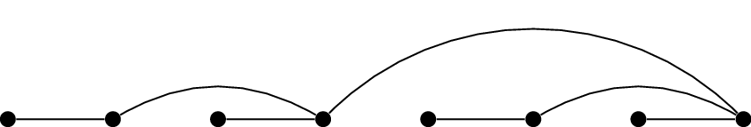
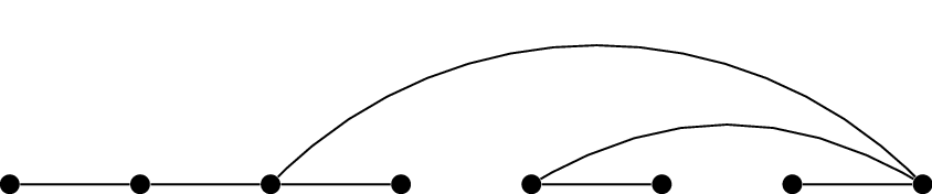
A bad vertex orderingA good vertex ordering
Two ways to order the vertices of a tree before coloring it
greedily
More importantly, we should give the vertices an order: the order in
which we color them. This choice is vitally important to the outcome.
Consider the two diagrams in Figure 19.2,
which show the same tree (or isomorphic trees). Of course, we know that
the tree is \(2\)-colorable, because
all trees are bipartite—but the greedy algorithm doesn’t know!
What happens if you greedily color the
vertices of the tree by going left to right in Figure 19.2(a)?
The colors used will be \(1, 2, 1, 3, 1, 2, 1, 4\) in that order; we
use \(4\) colors.
What happens if you greedily color the
vertices of the tree by going left to right in Figure 19.2(b)?
The colors used will be \(1, 2, 1, 2, 1, 2, 1, 2\) in that order; we
use \(2\) colors.
In the practice problems at the end of this chapter, I will ask a few
more questions about these examples. To summarize, if the vertices are
ordered badly, then the greedy algorithm can color even a tree with
arbitrarily many colors. However, if you know an optimal way to color a
graph ahead of time, you can always convince the greedy algorithm to do
just as well. Finding a good way to order the vertices without knowing
the answer in advance is the hard part.
Even if we don’t have a good idea for how to order the vertices,
though, there are some worst-case guarantees.
Proposition 19.1. Any graph \(G\) with maximum degree \(\Delta(G)\) is \((\Delta(G)+1)\)-colorable.
Proof. Give the vertex set \(V(G)\) an arbitrary order \(x_1, x_2, \dots, x_n\), and color \(G\) using the greedy algorithm, using the
positive integers as the set of colors.
For each \(i\), when the greedy
algorithm gets to vertex \(x_i\), that
vertex has at most \(\Delta(G)\)
neighbors among \(x_1, x_2, \dots,
x_{i-1}\). At most \(\Delta(G)\)
different colors can be represented on those neighbors. Therefore, at
least one of the colors \(1, 2, \dots,
\Delta(G)+1\) does not appear on any of \(x_i\)’s neighbors.
The greedy algorithm will never use a number higher than \(\Delta(G)+1\) if a lower one is available,
so it will give \(x_i\) some color from
the set \(\{1, 2, \dots,
\Delta(G)+1\}\). This is true for each \(i\), so at the end, the greedy algorithm
has found a coloring using at most \(\Delta(G)+1\) colors. ◻
The bound of Proposition 19.1 is better than having
no bound at all, but it’s not very good. However, that does not mean
that the greedy algorithm is no good! In this chapter and later in the
book, we will see examples where we can deduce better upper bounds from
the greedy algorithm for specific families of graphs. To do this, we
will use the structure of those graphs to come up with a better ordering
of the vertices.
(Of course, there are also proofs based on more sophisticated
algorithms.)
Two lower bounds
If we want to know the chromatic number of any graph for certain,
it’s not enough to find a coloring: we must also prove that we used the
least number of colors possible. To do this, we need lower bounds.
Unfortunately, a typical answer to why a graph is not \(7\)-colorable (for example) might be, “We
tried all possible ways to color the vertices, by making guesses and
backtracking and trying something else when they were wrong, and never
arrived at a \(7\)-coloring of the
entire graph.” State-of-the-art techniques might combine this with a
sequence of partial deductions of a standard type, but these are outside
the scope of this textbook and can still be exponentially long in some
cases.
In order to make something resembling progress, we will need to lower
our standards considerably. First, we will accept lower bounds that are
often far from the truth, in the hope that sometimes they will still
help us. Second, we will accept lower bounds that are themselves
difficult to find, as long as they provide us with a short proof of a
lower bound. This is more useful in theoretical problems, where we can
generalize that proof to deal with a family of graphs at once.
To arrive at the first such lower bound, we begin by asking: what’s
the most straightforward graph that requires \(k\) colors? It is the complete graph \(K_k\): its \(k\) vertices are all adjacent, so all of
them need different colors.
Moreover, if a large graph \(G\)
contains a copy of \(K_k\) inside it,
then we know that \(\chi(G) \ge k\) as
well. Even the copy of \(K_k\) inside
\(G\) needs \(k\) colors: coloring the other vertices can
only make things worse. (In general, if \(H\) is a subgraph of \(G\), then \(\chi(G) \ge \chi(H)\), because to color
\(G\), we must first color \(H\).)
Copies of \(K_k\) inside \(G\) correspond to \(k\)-vertex cliques. The size of the largest
clique in \(G\) is the clique number
\(\omega(G)\). We conclude:
Proposition 19.2. For any graph \(G\), \(\chi(G)
\ge \omega(G)\).
To be honest, I suspect that I don’t need to work hard to prove to
you that Proposition 19.2 is true. The
difficult thing for most people to accept—and we will see later in this
book that this has been difficult for serious mathematicians as well as
beginners in graph theory—is that Proposition 19.2 does not tell us
everything: that \(\chi(G)\) is not
always equal to \(\omega(G)\).
To see why this is true, we can start by understanding when \(\chi(G)\ge 3\), because another way to say
“\(\chi(G) \ge 3\)” is “\(G\) is not bipartite”, and we already know
a lot about bipartite graphs.
What does Proposition 19.2 say about when a
graph is not bipartite?
It says that \(\chi(G) \ge 3\) whenever \(\omega(G) \ge 3\): that \(G\) is not bipartite whenever \(G\) contains a copy of \(K_3\).
What do we already know about subgraphs
that mean a graph is not bipartite?
By Theorem 13.1, such subgraphs are
copies of \(C_3, C_5, C_7, C_9,
\dots\): cycles of odd length.
Of these graphs, \(C_3\) is
isomorphic to \(K_3\): in both cases,
we have three vertices, and any two are adjacent. So we might say that
Proposition 19.2 identifies the
smallest fundamental non-bipartite graph, but misses all the rest.
For a higher number of colors, the reality is even more complicated,
and Proposition 19.2 is even more of an
oversimplification. Still, it is a useful lower bound that is often
correct in practice.
What else can we use?
The independence number \(\alpha(G)\) is the exact opposite of the
clique number \(\omega(G)\): it is the
size of the largest set of vertices with no edges between them. So it
may seem surprising that the independence number can also help us put
lower bounds on the chromatic number.
= + +
A \(3\)-coloring of a graph
viewed as a partition into color classes
To see the connection, we switch to thinking of a coloring as a
partition into color classes; Figure 19.3
shows an example of such a partition. We started with the definition
that a coloring is proper when the endpoints of any edge are in
different color classes; however, another way to say this is that no two
vertices in the same color class are adjacent. In other words, a
coloring is proper if and only if every color class is an independent
set.
The independence number \(\alpha(G)\) tells us how big such color
classes can get, and we can use this to deduce another lower bound on
the chromatic number of \(G\).
Proposition 19.3. For any \(n\)-vertex graph \(G\), \(\chi(G)
\ge \frac{n}{\alpha(G)}\).
Proof. The independence number \(\alpha(G)\) is the largest number of
vertices in any independent set, so in particular every color class in a
\(k\)-coloring has at most \(\alpha(G)\) vertices. Together, the \(k\) color classes contain at most \(k \cdot \alpha(G)\) vertices. Every vertex
must be in one of the color classes, so if there are \(n\) vertices, then \(k \cdot \alpha(G) \ge n\). Rearranging, we
get \(k \ge
\frac{n}{\alpha(G)}\). ◻
If Proposition 19.3 and not
Proposition 19.2 is the reason why the
chromatic number of a graph is large, then this could be a very subtle
reason. We might not notice, when coloring a small portion of the graph,
that there is a problem; the effect of having no large independent sets
is only noticeable when we look at the graph as a whole.
But is this scenario actually possible? Are there graphs \(G\) where the independence number, and not
the clique number, controls \(\chi(G)\)?
In fact, not only do such graphs exist, but they are very common. In
Chapter 18, we explored what happens
when a graph on \(1 000 000\) vertices
is constructed by flipping coins to for each possible edge to decide if
we include it. We discovered that it is extremely unlikely for this
graph to have cliques or independent sets with more than \(40\) vertices.
If there are no cliques with more than
\(40\) vertices, the best we could hope
is a lower bound of \(\chi(G) \ge 40\),
and we might not even be able to get that.
If there are \(1
000 000\) vertices, but there are no independent sets of more
than \(40\) vertices, then at least
\(\frac{1 000 000}{40} = 25 000\)
colors are needed in a coloring.
By flipping a coin for every edge, we make every \(1 000 000\)-vertex graph equally likely.
This means that, if something is true with a very high probability for
this random graph, it is true for almost all \(1 000 000\)-vertex graphs. In other words,
\(\chi(G)\) is much larger than \(\omega(G)\) for almost all of these
graphs!
This does not mean, however, that Proposition 19.2 is useless. While
random graphs are a good source of examples, they do not actually
reflect most graphs we study: if a graph is interesting to us, there is
a good chance that it is atypical somehow. This example does not tell
the whole story.
In the rest of this chapter, we will see some alternative scenarios:
a class of graphs in which the lower bound of Proposition 19.2 always gives the
chromatic number exactly, and class of graphs in which the chromatic
number is much larger than both of our lower bounds.
Coloring interval graphs
In Chapter 18, we introduced interval
graphs: graphs obtained from a collection of intervals, with an edge
between vertices whenever the intervals overlap. These are a nice
application of graph coloring for two reasons: first, coloring interval
graphs has useful practical applications, and second, it is easier than
the general graph coloring problem.
First, on the applications. Suppose that the intervals we use to
build an interval graph are the start and end times of events: this is
the setting we looked at in Chapter 18.
We previously said that both cliques and independent sets have meaning
in this setting: cliques are sets of events all happening at the same
time, and independent sets are sets of events that don’t conflict with
each other.
Actually, there’s a subtlety: by
definition, a clique is a set of events where every pair has an overlap,
but does this mean that there’s a single point in time when all events
in the clique overlap?
Yes; to see this, take a clique of events,
let \(a\) be the first of these events
to end, and let \(z\) be the of these
events to start. Events \(a\) and \(z\) must overlap, because they’re part of a
clique together. At any time in that overlap, all events in the clique
have started (because even \(z\) has
started) but none have ended (because even \(a\) hasn’t ended).
The chromatic number of an interval graph is also a useful quantity.
Suppose we want to pick locations for the events. Two events happening
at the same time should be in different locations. At the same time, we
would like to use as few locations as possible: this makes it easier to
go from one event to another, and we might also have a limited number of
locations available. Choosing locations for the events is exactly a
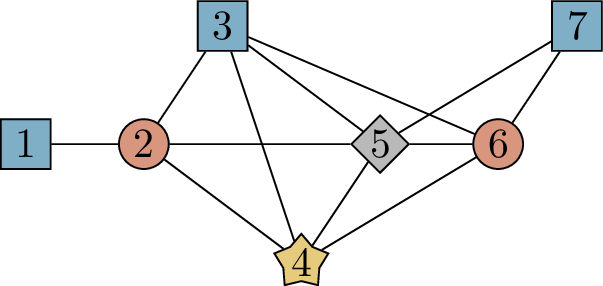
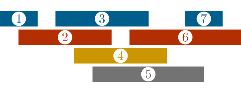
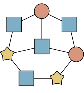
graph coloring problem, where the locations are the colors; Figure 19.4 shows a coloring of an
interval graph, and the corresponding solution to the scheduling problem
for the intervals.
A coloring of an interval graphSolving the scheduling problem
Coloring an interval graph
The same model can be useful in situations where the scheduling is
more metaphorical. For example, graph coloring can be used in the
register allocation problem in computer science [14]. Here, we want to assign the variables
used by a program to a limited supply of memory locations called
registers (if possible); however, two variables cannot be assigned to
the same register if they are in use at the same time. In simple
settings, the graph that represent conflicts between the variables
becomes an interval graph, and the assignment to registers is a coloring
of that interval graph.1
The interesting thing about coloring interval graphs is that the
complexity I alluded to in previous sections is almost not present. The
greedy algorithm is enough to color them optimally, and the lower bound
of Proposition 19.2 gives the exact
chromatic number, with no funny business.
Theorem 19.4. If \(G\) is an interval graph, then \(\chi(G) = \omega(G)\). Moreover, if the
greedy algorithm is given the vertices of \(G\) in order of the starting points of the
intervals, then it will use only \(\omega(G)\) colors.
Proof. The second half of the statement of the theorem is
actually all we need to prove. If the greedy algorithm uses only \(\omega(G)\) colors, then \(\chi(G) \le \omega(G)\); however, by
Proposition 19.2, \(\chi(G) \ge \omega(G)\), so the two must be
equal.
Let’s consider an iteration of the greedy algorithm in which it must
color a vertex \(x\) associated to
interval \([a,b]\). To see which colors
the algorithm cannot use, we look at the neighbors of \(x\) that already have a color. What are
these neighbors? They correspond to intervals that have an overlap
with \([a,b]\), but have starting
points less than \(a\).
In order to overlap \([a,b]\), these
intervals must contain the point \(a\).
This means that they all overlap each other, too! In fact, \(x\) and the neighbors of \(x\) already given a color must form a
clique: call this clique \(Q\).
There are \(|Q|-1\) neighbors of
\(x\) that have already been colored,
because the last element of \(Q\) is
\(x\) itself. Therefore at most \(|Q|-1\) colors are ruled out for \(x\), and the greedy algorithm will be able
to give \(x\) one of the first \(|Q|\) colors on its list.
The clique \(Q\) can be bigger or
smaller depending on \(x\), but in all
cases, \(|Q| \le \omega(G)\) by
definition of the clique number. Therefore the greedy algorithm always
uses one of the first \(\omega(G)\)
colors on the list, completing the proof. ◻
Mycielski graphs
We have already seen that in a randomly chosen graph, the chromatic
number can be much higher than the clique number. But the truth is even
worse than this: it is possible to increase the chromatic number
arbitrarily high while the clique number does not grow at all, and find
graphs where both Proposition 19.2 and Proposition 19.3 drastically
underestimate the chromatic number!
One method for doing this is a construction found in 1955 by Jan
Mycielski [76]. We
will first see it as an operation on graphs: a graph that transforms a
graph \(G\) into its Mycielskian \(M(G)\), increasing its chromatic number but
not its clique number. Then, the sequence of Mycielski graphs is
obtained by applying this operation over and over again.
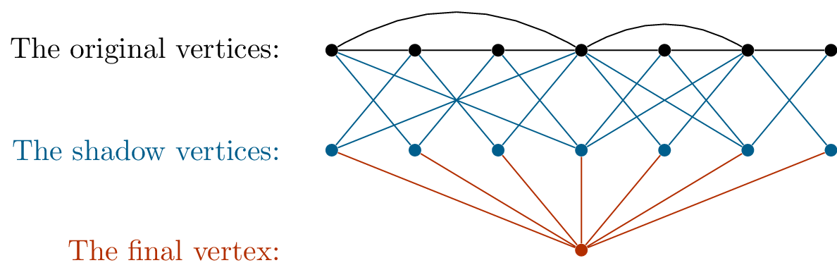
The Mycielskian\(M(G)\) of
a graph \(G\) is constructed in three
steps:
Start with a copy of \(G\). (I
will call the vertices in this copy of \(G\) the original vertices, for
ease of reference.)
For each original vertex \(x\),
add a new vertex \(x'\) adjacent to
the same original vertices as \(x\). (I
will call \(x'\) a shadow
vertex: the shadow of \(x\).) No
edges are added between the shadow vertices.
Finally, add one more vertex (which I will call the final
vertex) adjacent to all the shadow vertices.
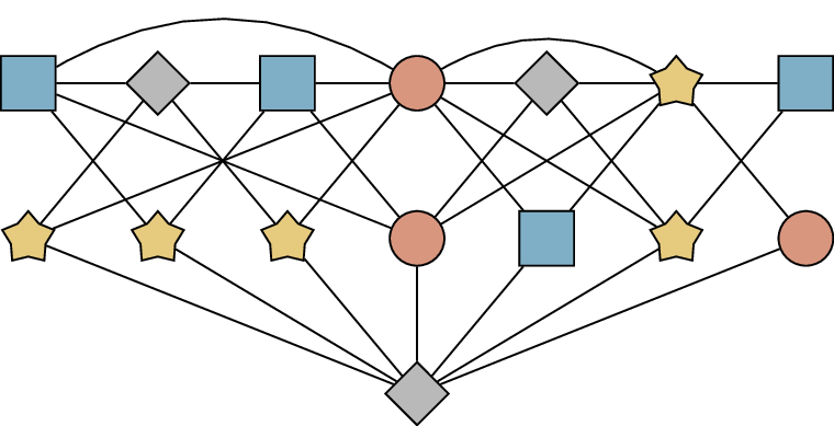
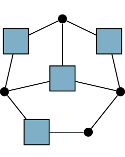
Figure 19.5 illustrates this construction
in an example. I should note that the terms “original vertices”, “shadow
vertices”, and “final vertex” are made up by me; there’s no standard
terminology.
The Mycielskian of a graph
The first objective of this definition is to avoid increasing the
clique number: we want \(\omega(M(G))\)
to stay equal to \(\omega(G)\).
Technically, this is violated when \(G\) has no edges: then \(\omega(G)=1\), but \(M(G)\) will gain some edges when the final
vertex is added, so \(\omega(M(G))=2\).
However, it will be true in all other cases.
Lemma 19.5. For all graphs \(G\) with \(\omega(G) \ge 2\), \(\omega(M(G)) = \omega(G)\).
Proof. We do not know anything about cliques formed by the
original vertices: these are cliques that already existed in \(G\). In particular, because \(M(G)\) contains a copy of \(G\), \(\omega(M(G))\) is at least \(\omega(G)\): every clique in \(G\) can also be found in \(M(G)\). It will also be possible that \(M(G)\) has new large cliques—but we will
show that none of these are bigger than cliques \(G\) already had.
To see this, suppose that \(Q\) is a
clique in \(M(G)\). If \(|Q| \le 2\), then we know that \(|Q| \le \omega(G)\) because we assumed
\(\omega(G) \ge 2\), so we may assume
that \(Q\) contains at least \(3\) vertices.
Can \(Q\)
contain the final vertex?
No, because none of the neighbors of the
final vertex are adjacent to each other.
Can \(Q\)
contain any shadow vertices?
Yes, but at most one: no two shadow
vertices are adjacent, so \(C\) cannot
contain two or more shadow vertices.
If \(Q\) contains no shadow vertices
at all, we are not interested: it’s contained in a copy of \(G\), therefore \(|Q| \le \omega(G)\). So suppose \(Q\) contains the original vertices \(x_1, x_2, \dots, x_{k-1}\) and the shadow
vertex \(x_k'\): the shadow of
\(x_k\). Since the original vertex
\(x_k\) is not adjacent to its
shadow \(x_k'\), we know that \(x_k \notin Q\).
By the construction of \(x_k'\),
among the original vertices, it has only the neighbors that \(x_k\) does: since \(x_k'\) is adjacent to \(x_1, x_2, \dots, x_{k-1}\), we know \(x_k\) must be adjacent to them, as well.
Therefore \(\{x_1, x_2, \dots, x_k\}\)
is also a clique, and it has the same number of vertices as \(Q\).
However, \(\{x_1, x_2, \dots,
x_k\}\) consists solely of original vertices, so it can have at
most \(\omega(G)\) vertices! This means
that \(|Q| \le \omega(G)\) as well.
We’ve now established the inequality \(|Q|
\le \omega(G)\) for all cliques \(Q\) in \(M(G)\), so we conclude that \(\omega(M(G)) \le \omega(G)\). This
concludes the proof. ◻
The most interesting case of Lemma 19.5
is when \(\omega(G) = 2\). (Such graphs
are sometimes called triangle-free graphs.) In this case, the graphs
\(M(G)\), \(M(M(G))\), and so on all have clique number
\(2\) as well: the least clique number
that a graph with edges can have.
Meanwhile, the chromatic number of \(G\) ticks up!
Lemma 19.6. For all graphs \(G\), \(\chi(M(G))
= \chi(G)+1\).
Proof. Here, we are expressing the solution to one
optimization problem (the chromatic number of \(M(G)\)) in terms of the solution to another
optimization problem (the chromatic number of \(G\)), so it’s worth thinking carefully
about what we need to prove.
To show that \(\chi(M(G)) \le
\chi(G)+1\), we need to show that \(M(G)\) has a coloring with \(\chi(G)+1\) colors. But we don’t need to
come up with the coloring of \(M(G)\)
from scratch: by definition of the chromatic number, we know that \(G\) has a \(\chi(G)\)-coloring, and we can use such a
coloring to help us.
We might imagine that to show that \(\chi(M(G)) \ge \chi(G)+1\), we need to show
that \(M(G)\) cannot be colored with
fewer colors, but proofs of impossibility are tricky: the paradigm of
turning one coloring into another is much friendlier. So we rewrite this
inequality as \(\chi(G) \le
\chi(M(G))-1\), and now we’re once again proving an upper bound
on a chromatic number. We need to show that \(G\) has a coloring with \(\chi(M(G))-1\) colors, and in the process,
we may use a \(\chi(M(G))\)-coloring of
\(M(G)\).
With the strategy talk out of the way, we can go on to the proof.
For the first step… I don’t like phrases like, “The obvious thing
will work,” because what’s obvious and what isn’t depends on your
experience. But the obvious thing will work. It’s okay if it doesn’t
feel obvious yet; use it to train your intuition so that future
arguments like it will be be more intuitive.
We start with a coloring of \(G\)
using \(\chi(G)\) colors. We would like
to color \(M(G)\) using only one more
color than that. Since \(M(G)\) starts
with a copy of \(G\) inside it, the
natural thing to do is to give every original vertex the same color as
in the \(\chi(G)\)-coloring of \(G\). Next, for each original vertex \(x\), give its shadow \(x'\) the same color as \(x\): this is guaranteed to work, because
the vertices adjacent to \(x'\) are
all original vertices adjacent to \(x\), so none of them can have the same
color as \(x\). For the final vertex,
use a new color we haven’t used yet.
The second step is harder. Let \(k =
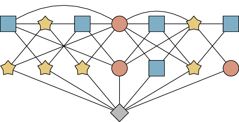
\chi(M(G))\), so that there is a \(k\)-coloring of \(M(G)\). We would like a coloring of \(G\) using only \(k-1\) colors. Inside our coloring of \(M(G)\), there is a coloring of \(G\)… but it may well use all \(k\) colors. Figure 19.6(a) shows an example, using the
same \(M(G)\) as in Figure 19.5.
A proper coloring of \(M(G)\)An improper coloring of \(M(G)\)
Going from a \(k\)-coloring
of \(M(G)\) to a \((k-1)\)-coloring of \(G\)
We want to modify this coloring so that it only uses \(k-1\) colors on the original vertices.
Motivated by our first step, we would like the color used on the final
vertex (let \(c\) be this color) to be
the color we get rid of. It’s a problem if any of the original vertices
have color \(c\); to “fix” it, whenever
an original vertex \(x\) is assigned
color \(c\), we give \(x\) the color of its shadow \(x'\).
What if the shadow \(x'\) is also assigned color \(c\)?
That’s impossible: \(x'\) is adjacent to the final vertex,
which has color \(c\), so \(x'\) must have some other color.
An example of the modified coloring we get is shown in Figure 19.6, and you can see from
this example that it might be an improper coloring. In Figure 19.6, an original vertex
recolored to is adjacent to two shadow vertices that also have color .
In general, when we give \(x\) the
color of \(x'\), there is no
guarantee that no neighbor of \(x\) has
this color.
If we’ve gotten an improper coloring, surely our attempt was a
failure? Not quite: remember, we only want a coloring of \(G\), not all of \(M(G)\). It turns out that if we only look
at the original vertices, the coloring we have is a proper coloring!
To see this, let \(x\) and \(y\) be two adjacent original vertices. If
neither \(x\) nor \(y\) had color \(c\), then the colors of \(x\) and \(y\) are unchanged from the \(k\)-coloring we started with, so the colors
of \(x\) and \(y\) are still different. It’s also not
possible that both \(x\) and \(y\) both had color \(c\); because we started with a proper \(k\)-coloring.
The last case is that only one of \(x\) and \(y\) (without loss of generality, \(x\)) had color \(c\). In this case, the color of \(x\) is changed to the color of \(x'\) in the \(k\)-coloring. By the construction of \(M(G)\), \(x'\) and \(y\) are also adjacent; therefore the color
of \(x'\) is not the same as the
color of \(y\). It follows that \(x\) and \(y\) still have different colors after the
change.
As a result, if we keep only the original vertices, then we do get a
proper \((k-1)\)-coloring of \(G\). Therefore \(\chi(G) \le k-1\); since \(k = \chi(M(G))\), this completes the second
step and concludes the proof of the theorem. ◻
Lemma 19.5 and Lemma 19.6 are the two properties of
the Mycielskian we needed to prove the following theorem.
Theorem 19.7. For all \(k\ge 1\), there exists a \(M_k\) with \(\omega(M_k) \le 2\) and \(\chi(M_k) = k\).
Proof. We induct on \(k\).
When \(k=1\) and when \(k=2\), a complete graph (\(K_1\) and \(K_2\), respectively) will do, so that’s
what we use for \(M_1\) and \(M_2\).
For the induction step, assume that we’ve already constructed a graph
\(M_{k-1}\) with \(\omega(M_{k-1}) \le 2\) and \(\chi(M_{k-1}) = k-1\). Let \(M_k = M(M_{k-1})\): the Mycielskian of
\(M_{k-1}\). By Lemma 19.5, \(\omega(M_k) \le 2\); by Lemma 19.6, \(\chi(M_k) = \chi(M_{k-1}) + 1 = k\). These
are exactly the two facts we needed to complete the induction step.
By induction, \(M_k\) exists for all
\(k\ge 1\). ◻
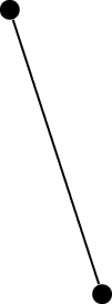
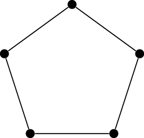
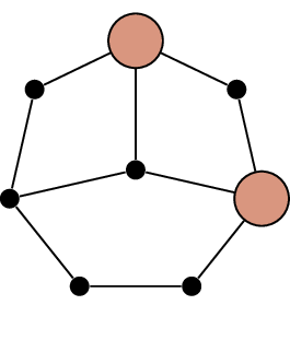
The graphs in the sequence \(M_2, M_3, M_4,
\dots\) are called the Mycielski graphs. (We rarely
include \(M_1\), because it is not
truly part of the recurrence: \(M_2\)
is not the Mycielskian of \(M_1\), but
a second base case.) Figure 19.7
shows the first few graphs in the sequence.
\(M_2\): the base
case\(M_3\): the \(5\)-cycle\(M_4\): the Grötzsch
graph
The first few graphs in the sequence of Mycielski
graphs
The graph \(M_3\) is isomorphic to
the cycle graph \(C_5\), though it
takes some “untwisting” to obtain a symmetric diagram from a 3-layer
diagram in the style of Figure 19.5.
Finally, let help you make sense of how we get from \(C_5\) to the diagram in Figure 19.7(c). The original vertices have
stayed in their place, with their shadows placed halfway to the center
of the diagram; the final vertex placed at the center. The resulting
graph, \(M_4\), is known as the
Grötzsch graph. It is named after Herbert Grötzsch, who used it in 1959
for the same purpose as Mycielski: as an example of a triangle-free
graph with chromatic number \(4\)[42].
Since the Mycielski graphs have clique
number \(2\), Proposition 19.2 does not give a good
lower bound on their chromatic number. What about Proposition 19.3?
It is almost no better: the shadow
vertices in \(M_k\) form an independent
set containing almost half of all the vertices. Therefore Proposition 19.3 only proves that
\(\chi(M_k) \ge 3\).
Practice problems
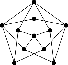
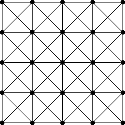
Let \(G\) be the \(25\)-vertex graph shown below:
What is the clique number \(\omega(G)\)? What lower bound on \(\chi(G)\) does it give?
What is the independence number \(\alpha(G)\)? What lower bound on \(\chi(G)\) does it give?
What is the maximum degree \(\Delta(G)\)? What upper bound on \(\chi(G)\) does it give?
What is the actual chromatic number of \(G\)?
Find a greedy coloring of the circulant graph \(\operatorname{Ci}_9(1,3)\), going through
its verticesin numerical order. Is there a coloring of \(\operatorname{Ci}_9(1,3)\) that uses fewer
colors than the greedy coloring you found?
Let \(G_n\) be the graph with
\(V(G_n) = \{1,2,\dots,3n\}\) in which
vertices \(x\) and \(y\) are adjacent if \(|x-y|\) is odd and not equal to \(1\).
If \(G_n\) is colored greedily
by going through the vertices in numerical order, how many colors are
used? Find the answer in terms of \(n\).
What is the chromatic number of \(G_n\), and why?
Alice and Bob take turns coloring the cube graph \(Q_3\), one vertex at a time. They have a
fixed set of colors \(C = \{\text{red},
\text{blue}, \text{yellow}\}\), and neither player is allowed to
give a vertex a color that has already been used on a neighbor of that
vertex. However, they have different goals: Alice (who goes first) wants
to get a coloring of \(Q_3\), while Bob
wants to arrive at a partial coloring which cannot be finished.
If both players play as well as possible, which player will
win?
Find a tree and a vertex ordering of that tree for which the
greedy algorithm will use \(5\)
different colors.
Prove that for all positive integers \(k\), there is a tree and a vertex ordering
of that tree for which the greedy algorithm will use \(k\) different colors.
The lowest-degree-last vertex ordering of an \(n\)-vertex graph \(G\) is constructed as follows, recursively.
We choose the last vertex, \(x_n\), to
be any vertex whose degree is the lowest degree in \(G\). To find the ordering \(x_1, x_2, \dots, x_{n-1}\) of the other
vertices, we find the lowest-degree-last ordering of the \((n-1)\)-vertex graph \(G - x_n\).
Prove that if \(G\) is a tree, then
the greedy coloring algorithm, using the lowest-degree-last ordering,
will never use more than \(2\)
colors.
Let \(G\) be a graph with
chromatic number \(k\), and let \(f \colon V(G) \to \{1,2,\dots,k\}\) be a
\(k\)-coloring of \(G\).
Prove that if we sort the vertices of \(G\) by their \(f\)-values (putting all vertices given
color \(1\) first and all the vertices
given color \(k\) last), then the
greedy algorithm will also find a \(k\)-coloring of \(G\).
(Be careful: if your proof shows that the greedy algorithm will find
the coloring \(f\) we started with,
then it’s wrong, because that claim is false in general.)
Suppose that the greedy algorithm uses \(k\) colors on a graph \(G\). Prove that \(G\) must have at least \(1 + 2 + \dots + (k-1) = \binom k2\)
edges.
Prove that if \(G\) has \(m\) edges, then \(\chi(G) \le 1 + \sqrt{2m}\).
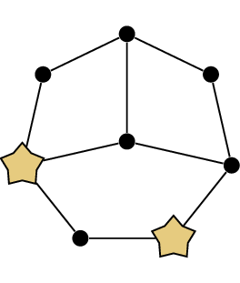
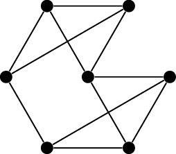
The graph below is called the Moser spindle. It is a
unit-distance graph: its vertices can be placed in the plane in such a
way that two vertices are adjacent exactly when they are at distance
\(1\) from each other.
Find a unit-distance drawing of the Moser spindle.
Prove that the Moser spindle has chromatic number \(4\).
The chromatic number of the plane is the least number of colors
needed to color every point of the plane so that no two points at
distance from each other are the same color. Leo and William Moser
constructed the Moser spindle in 1961 [75], proving that the chromatic number of the
plane is at least \(4\).
This was the best known lower bound until 2018, when Aubrey de Grey
constructed a \(1581\)-vertex unit
distance graph with chromatic number \(5\)[41].
The wheel graph with \(n\)
spokes is the graph obtained from the cycle graph \(C_{n}\) by adding a new vertex \(n+1\) adjacent to all \(n\) vertices of the cycle.
Draw a diagram of a wheel graph with \(5\) spokes.
Show that this graph has clique number \(3\) but chromatic number \(4\).
Generalize this construction to find a graph \(G\) in which \(\omega(G) = k\) but \(\chi(G)=k+1\), for every \(k \ge 3\).
It is interesting to think about coloring the co-bipartite
graphs: graphs whose complement is bipartite. A graph \(G\) is a co-bipartite graph if and only if
we can write \(V(G)\) as the disjoint
union of two sets \(A\) and \(B\) which are both cliques in \(G\) (and, additionally, there may be some
edges between \(A\) and \(B\)).
Show that in any coloring of a co-bipartite graph, each color
class contains at most \(2\)
vertices.
Suppose that a co-bipartite graph \(G\) has a coloring where \(k\) of the color classes have \(2\) vertices.
How else can you describe those \(k\) color classes, and their role in the
complement graph \(\overline G\) (a
bipartite graph)?
What is the connection between a clique in a co-bipartite graph
\(G\) and a vertex cover in its
complement \(\overline G\)?
Use parts (a)–(c) to prove that if \(G\) is a co-bipartite graph, then \(\chi(G) = \omega(G)\).
The following inequality is true whenever \(n_1, n_2, \dots, n_k\) are positive
integers with \(n_1 + n_2 + \dots + n_k =
n\): \[\sum_{i=1}^k \binom{n_i}{2} \ge
k \binom{n/k}{2} = \frac{n(n-k)}{2k}.\] Use this inequality to
find the maximum number of edges in an \(n\)-vertex graph with chromatic
number \(k\).
Footnotes
More sophisticated models can produce graphs with fewer
edges than the interval graph, with a smaller chromatic number that’s
harder to compute, but I will not get into those details.↩︎
 =
=  +
+  +
+