I’m hoping that the idea behind the definitions in this chapter feels
intuitive: that to measure the resilience of a graph, it makes sense to
see how much you have to remove from the graph to disconnect it. There
is a lot more to these definitions, and they turn out to have
connections to all parts of graph theory. However, it’s going to take a
bit of time to get there, and the content of this chapter is mostly
setup.
When I’ve taught this material in the past, I’ve sometimes focused
only on vertex connectivity and not on edge connectivity, for reasons of
time. If you do have the time, I think it is nice to look at both,
because the contrast helps you understand the logic of each case. For
example, if it’s hard at first to see why internally disjoint paths are
what we need for lower bounds on \(\kappa(s,t)\), then edge-disjoint paths and
their lower bounds on \(\kappa'(s,t)\) provide a second example
of the same idea for comparison.
The final section on duality is a topic I could have discussed
earlier in the book, but now we have lots of examples to look back to. I
should note that in graph theory, duality is a relationship between
optimization problems that just sometimes appears; we will occasionally
prove it appears, but not explain why. Using linear programming, we
could obtain more of an explanation, and even deduce what the correct
duals of some optimization problems should be without seeing them
before. That would take us too far afield, though.
Vertex and edge cuts
In the previous chapter, we defined cut vertices and \(2\)-connected graphs; much earlier in the
book, we defined bridges. In this chapter, we will discuss
generalizations of all three definitions.
We begin with the definition of a vertex cut in a
graph \(G\). This is subset \(U \subseteq V(G)\) such that when all
vertices in \(U\) are deleted, the
remaining graph \(G-U\) is not
connected.
Don’t confuse “vertex cut” and “cut vertex”, though they have the
same words in a different order! A cut vertex is a vertex, with “cut” as
the adjective: it is a vertex which cuts. A vertex cut is a cut (as in,
“I sliced the cake in half with a single cut”), with “vertex” as the
adjective: it is a cut made up of vertices.
The two terms are related, though. If \(G\) is a connected graph, a vertex \(x\) is a cut vertex of \(G\) if and only if the set \(\{x\}\) is a vertex cut of \(G\).
What if \(G\) is not connected?
In this case, cut vertices are those that
increase the number of connected components. Meanwhile, \(\{x\}\) is almost always a vertex cut; the
exception is when \(x\) is an isolated
vertex and the rest of the graph is connected.
Usually, this will not matter, because we will be looking for the
smallest vertex cuts we can. If \(G\)
is not connected, we will simply say that \(\varnothing\) (the empty set) is a vertex
cut.
Making vertex cuts an optimization problem in this way makes sense,
because it is not surprising when we disconnect a graph by deleting many
vertices. We ask: what is the least number of vertices whose deletion
disconnects the graph? Unfortunately, before we make that into a
definition, we have to tackle an awkward obstacle.
Is it always possible to disconnect a
graph by deleting enough vertices?
Almost always, except for complete
graphs!
In \(K_n\), any two vertices are
adjacent, and will remain adjacent no matter how many other vertices we
remove. This means that (aside from the question of what happens if we
delete every single vertex) we can’t disconnect \(K_n\) by deleting some of its vertices:
\(K_n\) has no vertex cuts.
This is related to what happened with \(2\)-connected graphs in the previous
chapter: we didn’t want \(K_2\) to be
\(2\)-connected, because most of the
theorems about \(2\)-connected graphs
do not apply to it, so we specifically excluded it from the
definition.
Accordingly, we define the connectivity (or
vertex connectivity) \(\kappa(G)\) of a graph \(G\) to be the smallest number of vertices
in a vertex cut of \(G\), if such a
vertex cut exists. If not, then \(G\)
is isomorphic to \(K_n\) for some \(n\), and we “artificially” define \(\kappa(K_n) = n-1\).
We also say that a graph \(G\) is
\(k\)-connected if
\(\kappa(G) \ge k\). This is in line
with our previous definitions. For graphs with at least \(2\) vertices, “\(1\)-connected” and “connected” are
synonyms; meanwhile, \(2\)-connected
graphs (as defined in Chapter 25) still have the
same definition if we set \(k=2\) in
the definition of \(k\)-connected
graph.
Why does the definition of \(k\)-connected graphs have an inequality:
\(\kappa(G) \ge k\), rather than \(\kappa(G)=k\)?
We say “\(G\) is \(k\)-connected” when we want to say that
\(G\) is connected enough for something
to work. For example, all \(2\)-connected graphs have ear
decompositions, even if they are also \(3\)-connected or \(100\)-connected.
This is similar to the way we defined \(k\)-colorable graphs: they are the graphs
with \(\chi(G) \le k\).
We must specify “vertex cut” and we often specify “vertex
connectivity” because all of these definitions have an equivalent for
deleting edges, rather than vertices, of a graph. The story is almost
the same for edges, so I will just present all the definitions at
once.
An edge cut in a graph \(G\) is a subset \(X \subseteq E(G)\) such that when all edges
in \(X\) are deleted, the remaining
graph \(G-X\) is not connected.
The edge connectivity of \(G\), denoted \(\kappa'(G)\), is the smallest number of
edges in an edge cut of \(G\), if \(G\) has at least two vertices. If \(G\) has only one vertex, then we set \(\kappa'(G)=0\).
Finally, a graph \(G\) is
\(k\)-edge-connected
if \(\kappa'(G) \ge k\).
Do we need to take any special care when
\(G = K_n\)?
Not unless \(n=1\) (which the definition addresses).
When \(G\) at least \(2\) vertices, it is always possible to
disconnect \(G\) by deleting some
edges: in particular, deleting all edges would be enough.
In Chapter 20, we discussed the correspondence
between “vertex versions” and “edge versions” of a problem, and used the
same notation: for example, \(\alpha'(G)\) and \(\chi'(G)\) are the edge versions of
\(\alpha(G)\) and \(\chi(G)\). I will use the same notation
here. In other sources, \(\lambda(G)\)
is also a common notation for edge connectivity, but I’d rather not make
you memorize even more Greek letters.
Often the edge version of a problem is
just the vertex version, but applied to the line graph \(L(G)\) rather than \(G\). Is that true here—is \(\kappa'(G) = \kappa(L(G))\)?
Not quite. I leave the details to practice
problem, but a relationship exists only in one direction: \(\kappa'(G) \le \kappa(L(G))\).
Let \(X\) be an edge cut in \(G\), and let \(S\) be the set of vertices in one connected
component of \(G-X\). Then \(X\) must contain all edges of \(G\) with one endpoint in \(S\) and one endpoint in \(V(G)-S\). Though \(X\) could contain other edges, this is
wasteful: just deleting all the edges between \(S\) and \(V(G)-S\) is enough to disconnect \(G\).
Accordingly, for \(S \subseteq
V(G)\), we define the edge boundary of \(S\) to be the set of all edges of \(G\) with exactly one endpoint in \(S\). We denote it \(\partial_G(S)\) or just \(\partial(S)\) when the graph \(G\) does not need to be specified.
Suppose \(X\) is a minimum edge cut,
or even a minimal one (by the distinction described in
Chapter 13): we cannot remove any
edges from \(X\) and still have an edge
cut. In that case, \(X = \partial(S)\)
for some \(S\). Another way to phrase
this is the following proposition:
Proposition 26.1. Every edge cut \(X\) in a connected graph contains an edge
boundary \(\partial_G(S)\) for some set
of vertices \(S\) that is neither \(\varnothing\) nor all of \(V(G)\). In particular, \(\kappa'(G)\) can be computed as the
minimum size \(|\partial_G(S)|\) of all
such edge boundaries.
We do not consider \(S =
\varnothing\) or \(S = V(G)\)
because these are the two cases that can never be a connected component
of \(G-X\), when \(X\) is an edge cut.
Is every set of the form \(\partial(S)\) a minimal edge cut?
No: it’s possible that \(\partial(S)\) contains a smaller edge cut
of the form \(\partial(T)\) for a
different set \(T\). For an extreme
example, consider a bipartite graph with bipartition \((A,B)\). Then the edges \(\partial(A)\) we need to separate \(A\) from \(B\) are all the edges of \(G\); the set \(\partial(\{x\})\) for a single vertex \(x\) can be much smaller.
Some examples
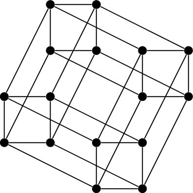
In Chapter 25, we saw that the
cube graph \(Q_3\) is \(2\)-connected. In fact, we can go one step
further.
Proposition 26.2. \(\kappa(Q_3) = 3\).
Proof. Ear decompositions are a nice way to prove that
graphs are \(2\)-connected, but we
don’t yet have an equally nice way to show that graphs are \(3\)-connected. We will find one later in
this chapter, but for now, let’s resort to trickery.
We know \(Q_3\) has no cut vertex;
does it have a cut \(\{x,y\}\) of size
\(2\)? If it did, then in \(Q_3 - x\), vertex \(y\) would be a cut vertex: deleting it
would bring us to \(Q_3 - \{x,y\}\),
which by assumption is not connected. So we can check for this
possibility by checking whether \(Q_3 -
x\) is \(2\)-connected.
Normally, we’d have to do this by checking \(8\) possibilities for \(x\). In the case of the cube graph, there
are enough symmetries (automorphisms of the cube graph) that it’s enough
to check one vertex: all \(8\) cases
will be identical.
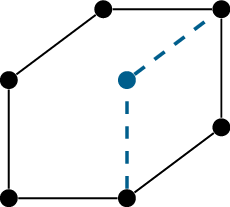
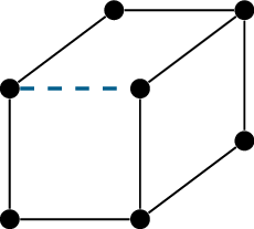
An ear decomposition of \(Q_3 -
x\)A vertex cut in \(Q_3\)
Determining the connectivity of the cube graph
Figure 26.1(a) shows an ear
decomposition of \(Q_3 - x\) for an
arbitrary vertex \(x\). (Well, it’s
only arbitrary mathematically; I deleted the vertex “in the back” of the
cube to make the diagram look nicer.) This shows that \(Q_3 - x\) is \(2\)-connected, so \(Q_3\) is \(3\)-connected.
Can it be \(4\)-connected? No,
because \(Q_3\) has a \(3\)-vertex cut, shown in Figure 26.1(b). Therefore \(\kappa(Q_3)\) is exactly \(3\). ◻
The vertex cut we chose in Figure 26.1(b) is
rather boring; we’ve disconnected a single vertex from the rest of the
graph. Such a vertex cut is possible in every graph \(G\), except in the unfortunate case of (you
guessed it) complete graphs. By deleting all edges incident to a vertex
\(x\), we also disconnect \(x\) from the rest of \(G\), so there is an edge cut of this type
as well. To make the cuts as small as possible, we want to choose a
vertex \(x\) of degree \(\delta(G)\): the minimum degree of \(G\).
This is not universal; we wouldn’t study connectivity if it always
turned out to be equal to the minimum degree. However, the following
relationship (also proved by Whitney, like most of the results in
Chapter 25) always
holds:
Theorem 26.3. For any graph \(G\), \(\kappa(G)
\le \kappa'(G) \le \delta(G)\).
Proof. The second inequality, \(\kappa'(G) \le \delta(G)\), follows
from our discussion just before the theorem: if \(x\) is a vertex of degree \(\delta(G)\), then deleting all \(\delta(G)\) edges incident to \(x\) will disconnect \(x\) from the rest of the graph, so it is
always an edge cut. (As usual with optimization problems, finding a
particular solution gives us an inequality, because there might be
better solutions.)
The more difficult inequality is the first. To prove that \(\kappa(G) \le \kappa'(G)\), we need to
do the following: given an edge cut \(X\) of size \(\kappa'(G)\), find a vertex cut \(U\) with \(|U|
\le |X|\). By Proposition 26.1,
we can assume that \(X =
\partial_G(S)\) for some set \(S\) such that \(\varnothing \ne S \subsetneq V(G)\).
I like the proof of this inequality because it is an excellent
exercise in attempting an argument, identifying the holes in it, and
then patching the holes. A few rounds of this, and we will have a
complete proof.
Let’s begin with the following strategy: to find \(U\), go through the edges in \(\partial(S)\), and for each \(xy \in \partial(S)\), add either \(x\) or \(y\) to \(U\). Deleting an endpoint of \(xy\) also deletes the edge \(xy\), so after these deletions, \(S\) (or what’s left of it) is disconnected
from the rest of the graph.
What could go wrong?
It’s possible that in deleting these
endpoints, we’ve actually deleted every vertex in \(S\), or every vertex not in \(S\), so the remaining graph is still
connected.
Okay, so let’s make sure that we avoid this. Begin by picking a
vertex \(s \in S\) and a vertex \(t \notin S\). For every edge \(xy \in \partial(S)\), add either \(x\) or \(y\) to \(U\), but with a restriction: if \(x=s\), add \(y\) to \(U\), and if \(y=t\), add \(x\) to \(U\). Then in \(G-U\), there is no way to get from \(s\) to \(t\), because \(s
\in S\), \(t\notin S\), and we
have destroyed all edges leaving \(S\).
What could go wrong?
The restriction we’ve added doesn’t leave
us an option to choose if one of the edges in \(\partial(S)\) is the edge \(st\).
Okay, fair enough; let’s make sure that we pick a vertex \(s \in S\) and a vertex \(t \notin S\) that are not adjacent.
What could go wrong?
Maybe every vertex in \(S\) is adjacent to every vertex not in
\(S\), so that no such \(s\) and \(t\) can be picked.
This is a surprising situation to be in! Let \(G\) have \(n\) vertices, and let \(|S|=k\). Then \(\partial(S)\) contains all edges between
the \(k\) vertices in \(S\) and the \(n-k\) vertices not in \(S\): this is a lot: \(|\partial(S)| = k(n-k)\). We have assumed
that \(\kappa'(G) = |\partial(S)| =
k(n-k)\), but in fact, \(k(n-k) >
n-1\) except when \(k=1\) or
\(k=n-1\).
Since we already know that \(\kappa'(G)
\le \delta(G)\), and in every \(n\)-vertex graph, \(\delta(G) \le n-1\), only one possibility
remains: \(\kappa'(G) = n-1 =
\delta(G)\).
What graph must \(G\) be?
\(G\)
must be isomorphic to \(K_n\); this is
the only \(n\)-vertex graph with
minimum degree \(n-1\).
When \(G\) is isomorphic to \(K_n\), \(\kappa'(G)=\delta(G)=n-1\), we’ve
defined \(\kappa(G)=n-1\) artificially
(and this theorem is part of the reason why). So the inequality \(\kappa(G) \le \kappa'(G)\) is
satisfied.
Now we just have to carry out our argument assuming \(G\) is not a copy of \(K_n\). This means that \(\delta(G) < n-1\), so \(\kappa'(G) < n-1\), so \(|\partial(S)| < n-1\). This means that
not all \(k(n-k)\) of the possible
edges with one endpoint in \(S\) are
actually present. Therefore we can choose \(s
\in S\) and \(t \notin S\) which
are not adjacent, and construct \(U\)
by the following rule: for each edge \(xy \in
\partial(S)\), add either \(x\)
or \(y\) to \(U\), taking care not to add either \(s\) or \(t\). As we’ve already shown, this is a
vertex cut of size at most \(|\partial(S)|\), proving that \(\kappa(G) \le \kappa'(G)\). ◻
Since this is a section called “Examples”, let me reassure you by
means of an example that apart from the constraint \(\kappa(G) \le \kappa'(G) \le
\delta(G)\), almost all triples \((\kappa(G), \kappa'(G), \delta(G))\)
are possible. There is only one other constraint on such triples: if
\(\kappa(G)=0\), it is because \(G\) is not connected, so \(\kappa'(G)=0\) as well.
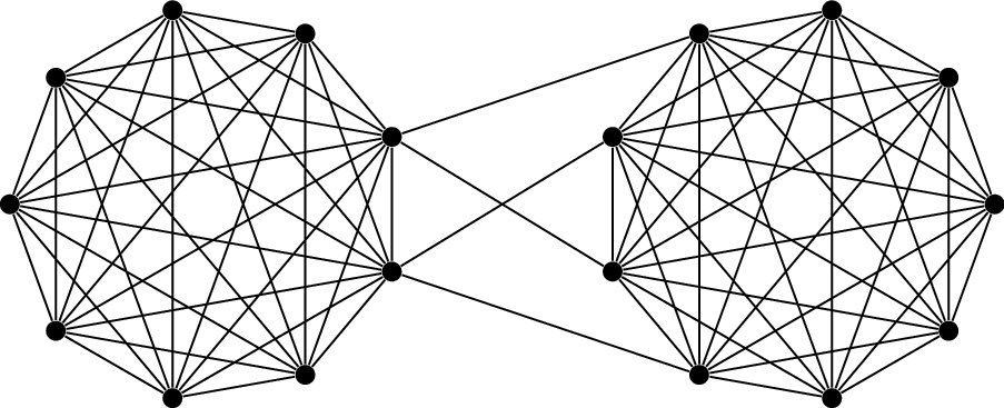
Let \(1 \le a \le b \le c\). To find
a graph where \(\kappa(G) = a\), \(\kappa'(G) = b\), and \(\delta(G) = c\), begin with two copies of
\(K_{c+1}\). Let \(A\) be a set of \(a\) vertices in the first copy and let
\(B\) be a set of \(b\) vertices in the second copy; add \(b\) edges between \(A\) and \(B\), making sure to use each vertex in
\(A\) at least once and each vertex in
\(B\) exactly once. Call the result
\(G_{a,b,c,d}\). An example of this
construction with \(a=2\), \(b=4\), and \(c=8\) is shown in Figure 26.2.
A graph with \(\kappa(G)=2\), \(\kappa'(G)=4\), and \(\delta(G)=8\)Why is \(\kappa(G_{a,b,c,d})=a\)?
The vertices in \(A\) are an \(a\)-vertex cut. If we delete fewer
than \(a\) vertices, we can find
vertices \(x \in A\) and \(y \in B\) that are adjacent, and have not
been deleted; since every vertex of \(G_{a,b,c,d}\) is adjacent to either \(x\) or \(y\), the graph will still be
connected.
Why is \(\kappa'(G_{a,b,c,d})=b\)?
The edges between \(A\) and \(B\) are a \(b\)-edge cut. If we delete fewer than \(b\) edges, then in particular (because
\(b \le c\), and \(\kappa'(K_{c+1}) = c\)) each copy of
\(K_{c+1}\) is connected; also, at
least one edge between the two copies of \(K_{c+1}\) remains, connecting them
together.
Why is \(\delta(G_{a,b,c,d})=c\)?
We started with two copies of \(K_{c+1}\), in which every vertex has
degree \(c\). We added edges to \(a+b\) vertices, which is at most \(2c\); therefore at least two vertices still
have degree \(c\).
Why is there even a \(d\) in \(G_{a,b,c,d}\)?
No reason; I’m just messing with you.
Local connectivity
We often want to solve a problem which is similar to finding a vertex
cut or edge cut in a graph, but more specialized.
As I’m writing this chapter, it is November, and in the United
States, Thanksgiving is coming up. Many people travel long distances to
celebrate Thanksgiving with their family, but it’s also almost winter,
so if you take a plane across the US, you might have to deal with
cancellations due to snow and other winter weather. Some flights might
be canceled, deleting an edge in the graph of possible airplane trips.
In extreme circumstances, an entire airport might shut down and divert
all flights, deleting a vertex.
How many of these events must happen for you to be entirely unable to
get to your destination? This is a bit like the question of computing
edge connectivity (in the case of flight cancellations) or vertex
connectivity (in the case of closed airports).
In practice, vertex and edge connectivity of this graph are low. I
can speak to this from personal experience: I have spent three years
living in Urbana, Illinois. The local airport has flights to only two
other airports: Chicago O’Hare and Dallas–Fort Worth. It was not a very
reliable means of travel, especially in the winter!
Suppose, however, that you live in New York City and your family
lives in Los Angeles. You do not care if a few cancellations are enough
to disconnect you from Urbana, because you’re not going to Urbana. In
your case, the number of cancellations that would have to occur for all
routes you could take to be blocked off is truly implausible.
To model situations like this, we need a more specialized definition.
Here, let \(s\) and \(t\) be two vertices in a graph \(G\); we will specifically consider what it
takes to separate \(s\) from \(t\).
An \(s-t\) vertex
cut (or just \(s-t\)
cut) in \(G\) is a vertex cut
\(U\) that separates \(s\) from \(t\): vertices \(s\) and \(t\) are in different connected components
of \(G-U\). (In particular, \(U\) must not contain either \(s\) or \(t\).)
The \(s-t\) connectivity in
\(G\), denoted \(\kappa_G(s,t)\) or just \(\kappa(s,t)\) if there is no need to
specify the graph, is the smallest number of vertices in an \(s-t\) cut.
An \(s-t\) edge
cut in \(G\) is an edge cut
\(X\) that separates \(s\) from \(t\): vertices \(s\) and \(t\) are in different connected components
of \(G-X\).
The \(s-t\) edge
connectivity in \(G\), denoted
\(\kappa'_G(s,t)\) or just \(\kappa(s,t)\), is the smallest number of
edges in an \(s-t\) edge cut.
What happens to \(\kappa(s,t)\) if \(s\) and \(t\) are adjacent?
In this case, there is no vertex cut that
separates \(s\) from \(t\); we either disregard this case entirely
or set \(\kappa(s,t) = \infty\).
However, there are no problems with defining \(\kappa'(s,t)\); we just have to make
sure that \(st\) is one of the edges we
delete.
There are, broadly speaking, two reasons to care about \(s-t\) cuts of the two types. One reason is
an application such as your hypothetical Thanksgiving travel plans from
New York City to Los Angeles, where you really only care about whether
an \(s-t\) path survives. There is
another: as we will discover in the next few chapters, finding \(\kappa_G(s,t)\) is sometimes much easier
than finding \(\kappa(G)\). If we
really want to know \(\kappa(G)\), we
might perform several computations of \(\kappa_G(s,t)\) instead.
If you were given a table of \(\kappa_G(s,t)\) and \(\kappa'_G(s,t)\) for all pairs of
vertices \(s\) and \(t\), could you use it to determine \(\kappa(G)\) and \(\kappa'(G)\)?
Yes \(\kappa'(G)\) is the minimum of \(\kappa'_G(s,t)\) over all pairs \(\{s,t\}\), and if \(G\) is not a complete graph, \(\kappa(G)\) is the minimum of \(\kappa_G(s,t)\) over all non-adjacent pairs
\(\{s,t\}\).
The quantities \(\kappa(s,t)\) and
\(\kappa'(s,t)\) are the solutions
to optimization problems: of all \(s-t\) cuts of the appropriate type, we want
to find the smallest. Finding upper bounds is, in both cases,
straightforward (if not necessarily easy): if you find an \(s-t\) cut \(U\), then you know that \(\kappa(s,t) \le |U|\). But how do we prove
a lower bound?
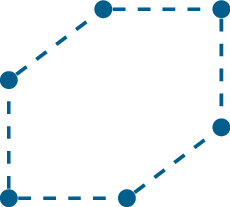
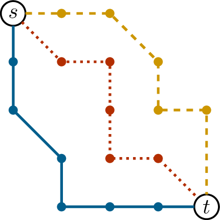
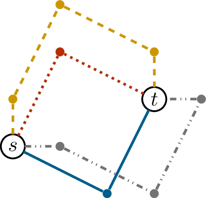
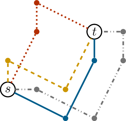
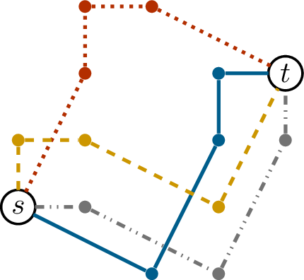
Internally disjoint pathsEdge-disjoint pathsJust some paths
Three different sets of three \(s-t\) paths
Here’s one possible answer. Suppose that the graph contains a
subgraph such as the one in Figure 26.3(a). It is the union
of three \(s-t\) paths (a blue path, a
red path, and a yellow path). Moreover, the three paths share no
internal vertices. Then it’s clear that \(\kappa(s,t) \ge 3\): we need to delete at
least one of the internal vertices from each path if we want to
disconnect \(s\) from \(t\).
Why is it important that the three paths
share no internal vertices?
Consider the paths in Figure 26.3(b), instead. They provide
three ways to get from \(s\) to \(t\), but some vertices are repeated. It’s
possible to destroy multiple paths by deleting just one vertex, and in
fact all three paths can be destroyed by deleting \(2\) vertices.
The paths in Figure 26.3(b) are still useful,
though: they share no edges. If we seek to disconnect \(s\) from \(t\) by deleting edges, the existence of
such paths proves that at least three edges need to be deleted: one from
each path. Compare this to the paths in Figure 26.3(c), which have no special
properties relative to each other! Here, we can destroy all three paths
by deleting just two edges.
To generalize, we say that two paths in a graph are
internally disjoint if they do not share any internal
vertices; they are edge-disjoint if they do not share
any edges. I want to emphasize that both of these definitions are
properties a pair of paths can have. It would not make sense to look at
an \(s-t\) path and ask, “Is this \(s-t\) path internally disjoint or not?”
For a set of paths, such as what we see in Figure 26.3, the formally correct phrasing
would be that the paths in a set are “pairwise internally disjoint” if
no two paths share internal vertices, and “pairwise edge-disjoint” if no
two paths share edges. The word “pairwise” emphasizes that we consider
the paths two at a time, rather than all at once; for a set of \(100\) paths, it’s not enough to know that
there’s no vertex that all \(100\)
paths pass through.
This is a mouthful. To make it a little bit easier, I will talk about
a “set of internally disjoint paths” or a “set of edge-disjoint paths”
to mean that any two paths in the set are internally disjoint or
edge-disjoint, respectively. In case you are confused, always think back
to this example and the argument we are trying to make with the set of
paths! We want the paths to be sufficiently separate that to destroy
them all (by deleting whichever of vertices or edges we’re thinking
about) we need to handle each path separately.
We will do a lot more with this idea in the next two chapters. For
now, I will use it to go one step further beyond Proposition 26.2.
Proposition 26.4. The hypercube graph \(Q_4\) is \(4\)-connected.
Proof. Our strategy will be to compute \(\kappa(Q_4)\) by computing \(\kappa(s,t)\) for every \(s\) and every \(t\). But first, let me begin with a bit of
review of \(Q_4\). This graph has \(2^4 = 16\) vertices, which are \(4\)-bit binary strings \(b_1b_2b_3b_4\). Two vertices are adjacent
if the binary strings agree in \(3\)
out of \(4\) positions, and only
disagree in \(1\) position.
The hypercube graph \(Q_4\) has many
automorphisms. To review some concepts you may not have thought about
since Chapter 2, I’ll write them
out in detail. We’ll need two types of automorphisms of \(Q_4\) to reduce the casework we have to
do:
For each position \(i\), let
\(\varphi_i \colon V(Q_4) \to V(Q_4)\)
be the function that flips the \(i\)th bit; for example, \(\varphi_3(0101) = 0111\). This is a
bijection because it is its own inverse. It is an automorphism because
when we compare two binary strings \(x\) and \(y\), if we flip the \(i\)th bit in both of them, it
doesn’t change which positions they agree in.
For every two positions \(i\)
and \(j\), let \(\varphi_{ij} \colon V(Q_4) \to V(Q_4)\) be
the function that swaps the \(i\)th and \(j\)th bits: for example, \(\varphi_{13}(1001) = 0011\). This is a
bijection because it is its own inverse. It is an automorphism because
when we compare two binary strings \(x\) and \(y\), applying \(\varphi_{ij}\) to both might move a
position they disagree in (from \(i\)
to \(j\) or from \(j\) to \(i\)) but won’t change the number of
disagreements.
Our goal is to compute \(\kappa(s,t)\) for every pair of vertices
\(\{s,t\}\). There are \(\binom{16}{2} = 90\) pairs to test if we do
it the hard way. However, by applying the automorphisms above, we can
reduce all \(90\) cases to just a few!
The general logic is this: if \(\varphi\) is any automorphism of \(Q_4\), then \(\kappa(s,t) = \kappa(\varphi(s),
\varphi(t))\).
How do we know this?
If there is a vertex cut \(U\) separating \(s\) from \(t\), then applying \(\varphi\) to its vertices gives a vertex
cut of the same size separating \(\varphi(s)\) from \(\varphi(t)\). In the other direction,
applying \(\varphi^{-1}\) to the
vertices of a \(\varphi(s)-\varphi(t)\)
cut gives an \(s-t\) cut of the same
size.
Consider any pair \(s,t \in
V(Q_4)\). First, some composition of the automorphisms \(\varphi_1, \dots, \varphi_4\) maps \(s\) to \(0000\) and \(t\) to some vertex \(t'\). Therefore \(\kappa(s,t) = \kappa(0000,t')\). The
second type of automorphisms (the \(\varphi_{ij}\)’s) leave \(0000\) unchanged, but some composition of
them sorts the bits of \(t'\) in
ascending order: to one of \(0001\),
\(0011\), \(0111\), or \(1111\). Therefore \[\kappa(Q_4) = \min\Big\{\kappa(0000,0001),\,
\kappa(0000,0011),\, \kappa(0000,0111),\, \kappa(0000,1111)
\Big\}.\] Of these four cases, \(\kappa(0000,0001) = \infty\) because \(0000\) and \(0001\) are adjacent; we can skip this one.
For the other three, the vertex cut \(\{0001,
0010, 0100, 1000\}\) consisting of all four neighbors of \(0000\) separates \(0000\) from the other vertices, so they are
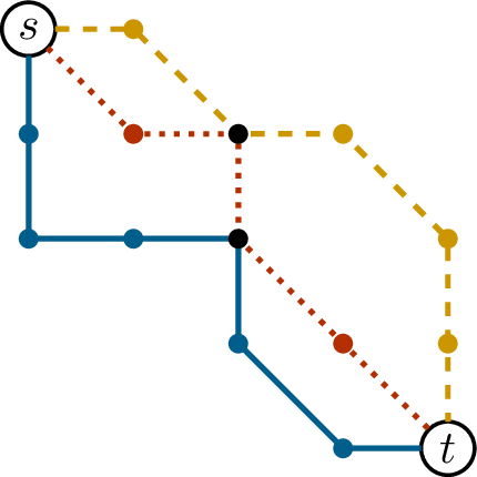
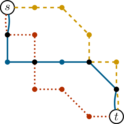
all at most \(4\). Finally, Figure 26.4 shows that in all three of
these cases, we can find a set of \(4\)
internally disjoint paths. Therefore \(4\) is a lower bound as well, and we
conclude that \(\kappa(Q_4) =
4\). ◻
What is \(\kappa'(Q_4)\)?
By Theorem 26.3, it
is sandwiched between \(\kappa(Q_4)\)
and \(\delta(Q_4)\). Both of these are
\(4\), so \(\kappa'(Q_4) = 4\) as well.
Duality
The technique of internally disjoint paths seems pretty powerful
based on this example, but there is an unresolved question. If we use
this technique to prove lower bounds on \(\kappa(s,t)\) or \(\kappa'(s,t)\), will we always be able
to prove a lower bound equal to the true value of these numbers? Or is
it possible that in some cases, \(\kappa(s,t)
= 4\), but the largest set of internally disjoint paths only
contains \(3\) paths?
In the next chapter, we will prove that this will never happen: not
for vertices, and not for edges. In preparation, let me tell you about
one framework to think about the relationship between \(s-t\) cuts and sets of disjoint paths:
optimization duality.
Optimization duality is a relationship that can exist between two
optimization problems: a maximization problem and a minimization
problem. We want to be fairly general here, but not so general that we
get lost in abstraction. Let’s say that:
The maximization problem is, given a set \(\mathcal X\) and a function \(f\colon \mathcal X \to \mathbb R\), to find
an element \(x \in \mathcal X\) such
that \(f(x)\) is as large as possible.
Written concisely, it is the problem of finding \(\max\{f(x) : x \in \mathcal X\}\).
The minimization problem is, given a set \(\mathcal Y\) and a function \(g \colon \mathcal Y \to \mathbb R\), to
find an element \(y \in \mathcal Y\)
such that \(g(y)\) is as small as
possible. Written concisely, it is the problem of finding \(\min\{g(y): y \in \mathcal Y\}\).
Let’s try putting some problems we’ve already studied into this
language. Don’t worry too much about how the functions \(f\) and \(g\) are implemented; it’s enough to know
they exist.
In the maximization problem of finding the
matching number of a graph \(G\), what
is \(\mathcal X\) and what is \(f\)?
The set \(\mathcal X\) is the set of all matchings in
\(G\). If \(x
\in \mathcal X\) is such a matching, then \(f(x)\) is the number of edges in it.
In the minimization problem of finding the
chromatic number of a graph \(G\), what
is \(\mathcal Y\) and what is \(g\)?
The set \(\mathcal Y\) is the set of all proper
colorings of \(G\). If \(y \in \mathcal Y\) is such a coloring, then
\(g(y)\) is the number of colors used
by \(y\).
Optimization duality comes in two forms: weak and strong. To begin
with, we say that a maximization problem \(\max\{f(x) : x \in \mathcal X\}\) and a
minimization problem \(\min\{g(y) : y \in
\mathcal Y\}\) are in weak duality if \(f(x) \ge g(y)\) for every \(x \in \mathcal X\) and every \(y \in \mathcal Y\). Equivalently, \[\max\{f(x) : x \in \mathcal X\} \le \min\{g(y) :
y \in \mathcal Y\}\] is the inequality that characterizes weak
duality.
Why is this helpful? Well, consider the example of matchings and
vertex covers in graphs: in the entire textbook, this is perhaps our
best example of dual optimization problems. By Proposition 13.4, whenever
\(M\) is a matching and \(U\) is a vertex cover in the same graph
\(G\), we have \(|E(M)| \le |U|\): the maximization problem
is always bounded above by the minimization problem. This means we can
try to find small vertex covers to get upper bounds on the size of a
matching: upper bounds that are otherwise hard to come by.
In general, duality fills a gap in our understanding of an
optimization problem. By default, if we have an optimization problem to
maximize \(f(x)\) over all \(x \in X\), and we’ve worked on it for a
while, we might not have anything to show for our progress except some
element \(x^* \in X\) for which \(f(x^*)\) is the largest found so far. This
proves a lower bound on the optimal value: \(\max\{f(x) : x \in \mathcal X\}\) is at
least \(f(x^*)\).
To prove an upper bound on \(\max\{f(x) : x
\in \mathcal X\}\), we could try every element of \(\mathcal X\) to see which is best. Or, we
could come up with and prove an insightful theorem that gives a general
upper bound. These both seem very hard. But if we have a dual problem
\(\min\{g(y) : y \in \mathcal Y\}\),
then we can switch to working on that problem, instead! After a while,
the element \(y^* \in Y\) for
which \(g(y^*)\) is the smallest found
so far is probably pretty good. This value \(g(y^*)\) will be an upper bound on our
original problem: by weak duality, \(\max\{f(x) : x \in \mathcal X\}\) is at
most \(g(y^*)\).
The reason weak duality is “weak” is that the bounds we get this way
might turn out to be very bad. Even if we’ve found the best \(x^*\) we can, weak duality does not
guarantee us a way to ever prove that it’s the best. If the two dual
problems meet in the middle, and \[\max\{f(x)
: x \in \mathcal X\} \le \min\{g(y) : y \in \mathcal Y\},\] we
say that they are in strong duality.
In the worst of all possible worlds, there is no structure to \(\mathcal X\), no meaning to \(f\), and no way to find \(\max\{f(x) : x \in \mathcal X\}\) except by
exhaustive search. In such a world, even if you find the optimal
solution \(x^*\) after hundreds of
hours of computing time, skeptics won’t trust you: they will say that
maybe your software had a bug in it, and you missed some cases. But with
strong duality,1 you can find an optimal solution
\(y^*\) to the dual problem. Now you
can silence the skeptics by simply checking that \(f(x^*) = g(y^*)\); this is a (hopefully)
quick way of demonstrating that both solutions are optimal.
Again, matchings and vertex covers are an ideal example, because the
duality here is sometimes, but not always strong.
When is there strong duality between
finding the largest matching in \(G\)
and finding the smallest vertex cover in \(G\)?
By Kőnig’s theorem (Theorem 14.2), strong duality holds when
\(G\) is bipartite.
(By the way, you should brush up on Kőnig’s theorem in preparation
for the next chapter; it will come in handy!)
So how does this apply to vertex and edge connectivity? The version
of the problem that exhibits duality is the problem with cuts and paths
between two specific vertices \(s\) and
\(t\); the “global” version is not as
nice.
Start with the problem of finding \(\kappa_G(s,t)\). This is a minimization
problem: we are looking for the smallest \(s-t\) cut in \(G\). The corresponding maximization problem
is the problem of finding the largest set of internally disjoint \(s-t\) paths. So far, we know:
Proposition 26.5. Let \(s\) and \(t\) be two vertices in a graph \(G\). If there is a set of \(k\) internally disjoint \(s-t\) paths in \(G\), then \(\kappa_G(s,t) \ge k\): there is no \(s-t\) cut with fewer than \(k\) vertices.
Proof. Take any set \(U\)
of fewer than \(k\) vertices, with
\(s,t \notin U\), that we suspect might
be an \(s-t\) cut. Every vertex \(x \in U\) lies on at most one of the \(s-t\) paths in our set, because they are
internally disjoint. There are \(k\)
paths, and fewer than \(k\) vertices in
\(U\), so there is at least one path
with no vertices of \(U\) on it.
That path still exists in \(G-U\),
proving that \(s\) and \(t\) are in the same connected component of
\(G-U\). So \(U\) is not an \(s-t\) cut, after all. ◻
Weak duality! The proposition gives an
inequality between the largest number of internally disjoint \(s-t\) paths and the smallest number of
vertices in an \(s-t\) cut, but it does
not guarantee that they meet in the middle. So far, we know of no reason
why there can’t be a graph \(G\) with
only \(10\) internally disjoint \(s-t\) paths, but no \(s-t\) cut with fewer than \(20\) vertices.
Similarly, we can prove weak duality between the minimization problem
of finding the smallest \(s-t\) edge
cut, and the maximization problem of finding the largest set of
edge-disjoint \(s-t\) paths:
Proposition 26.6. Let \(s\) and \(t\) be two vertices in a graph \(G\). If there is a set of \(k\) edge-disjoint \(s-t\) paths in \(G\), then \(\kappa'_G(s,t) \ge k\): there is no
\(s-t\) edge cut with fewer than \(k\) edges.
Proof. As before, but replacing vertices by edges. The key
point is that every edge in \(G\) lies
on at most one path in our set. A set of fewer than \(k\) edges cannot be an \(s-t\) edge cut, because one of our \(s-t\) paths will avoid it. ◻
Is there also weak duality between \(s-t\) edge cuts and internally disjoint
\(s-t\) paths?
Yes! Internally disjoint \(s-t\) paths are, in particular,
edge-disjoint.
But whether or not strong duality will hold, we’d like to aim for the
“least weak” weak duality, so we don’t want to restrict our maximization
problem unnecessarily. The most general sets of \(s-t\) paths that will work to give a lower
bound on \(\kappa'_G(s,t)\) are the
sets of edge-disjoint paths, so we want to use those.
In Chapter 27, we will prove that in both
cases, strong duality holds: a result known as Menger’s theorem.
Practice problems
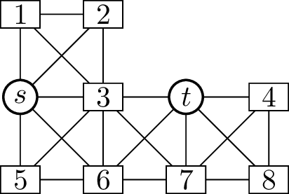
Let \(G\) be the graph shown
below.
Find the vertex connectivity \(\kappa(G)\).
Find the \(s-t\) edge
connectivity \(\kappa'_G(s,t)\).
Prove that \(\kappa(Q_4) = 4\)
directly: by showing that no set of \(3\) deleted vertices can disconnect \(Q_4\). Using Proposition 26.2 may help.
Prove that \(\kappa(Q_n) = n\)
by induction on \(n\), either directly
or using the idea of internally disjoint paths.
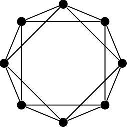
In Chapter 5, the Harary graph\(H_{n,r}\) was a particular circulant
graph we used in Theorem 5.1 to give an
example of an \(r\)-regular graph on
\(n\) vertices.
In fact, more is true: whenever \(0 \le r
\le n-1\) and at least one of \(r\) and \(n\) is even, the Harary graph \(H_{n,r}\) provides an example of an \(r\)-regular graph with \(\kappa(H_{n,r}) = r\). It achieves the
minimum possible number of edges in an \(r\)-connected \(n\)-vertex graph.
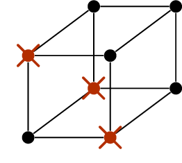
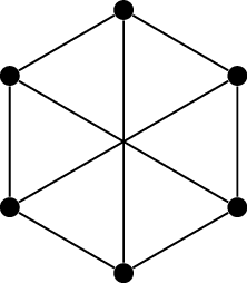
Prove that \(\kappa(H_{n,r}) =
r\) for all even \(n\) when
\(r=3\). The Harary graphs \(H_{6,3}\), \(H_{8,3}\), and \(H_{10,3}\) are shown as examples below:
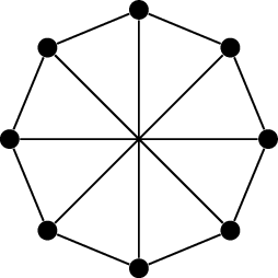
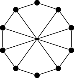
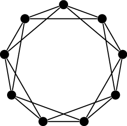
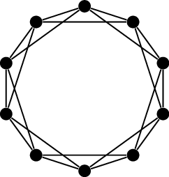
Prove that \(\kappa(H_{n,r}) =
r\) for all \(n\) when \(r=4\). The Harary graphs \(H_{8,4}\), \(H_{9,4}\), and \(H_{10,4}\) are shown as examples below:
If you are feeling confident, prove that \(\kappa(H_{n,r})=r\) for all valid choices
of \(n\) and \(r\).
Give an example of a connected \(r\)-regular circulant graph which is not
\(r\)-connected. (The smallest example
has \(8\) vertices.)
The Petersen graph is \(3\)-connected.
Prove this by picking two vertices of the Petersen graph that are
not adjacent, and finding a set of three internally disjoint paths
between them.
Prove this by picking a vertex of the Petersen graph, deleting
it, and finding an ear decomposition of the remaining graph.
Explain, using automorphisms of the Petersen graph, why either of
the strategies above is a fully general proof that the Petersen graph is
\(3\)-connected.
A graph is called fragile if it has a vertex cut which is an
independent set.
Prove that the clique number of a graph is \(2\), then it is fragile.
For all \(n \ge 3\), find an
example of a graph with \(n\) vertices
and \(2n-3\) edges which is not
fragile.
(This exercise is based on some observations in “A note on fragile
graphs” by Guantao Chen and Xingxing Yu [15].)
Let \(D\) be a strongly
connected digraph with at least \(3\) vertices (as defined in Chapter 12), and let \(G\) be its underlying graph (as
defined in Chapter 7). You may either
assume that \(D\) never contains both
arcs \((x,y)\) and \((y,x)\), or make \(G\) a multigraph with two copies of edge
\(xy\) in this case.
Prove that \(\kappa'(G) \ge
2\).
Give an example showing that it is not necessarily true that
\(\kappa(G) \ge 2\).
Without making use of symmetry, the strategy used to prove
Proposition 26.4 would seem hopeless,
because there are too many pairs \((s,t)\) for which \(\kappa(s,t)\) needs to be verified.
However, it is often enough to check a smaller, but well-chosen set of
pairs. The following strategy is due to Abdol Esfahanian and
S. L. Hakimi [31].
Let \(x\) be an arbitrary vertex of
a graph \(G\) which is not complete,
and suppose that the following is true:
For every vertex \(y\) not
adjacent to \(x\), \(\kappa_G(x,y) \ge k\).
For every two vertices \(y,z\)
that are adjacent to \(x\) but not to
each other, \(\kappa_G(y,z) \ge
k\).
Prove that \(\kappa(G) \ge
k\).
It is tempting to guess that the edge connectivity \(\kappa'(G)\) is equal to \(\kappa(L(G))\): the vertex connectivity of
the line graph of \(G\). However, this
is false.
Prove that every vertex cut in \(L(G)\) corresponds to an edge cut in \(G\). Deduce that \(\kappa'(G) \le \kappa(L(G))\).
Not every edge cut in \(G\) is a
vertex cut in \(L(G)\). Think about how
this statement might fail, and use it to find an example where \(\kappa'(G) < \kappa(L(G))\). (A
relatively small example exists with \(5\) vertices and \(8\) edges.)
Is there a way to compute \(\kappa'(G)\) using only \(\kappa(L(G))\) and some simple information
about \(G\)?
Footnotes
And possibly hundreds of hours more of computing time.↩︎