The focus of this chapter betrays my interests: more than half of it
has ended up related to Ramsey numbers and Ramsey’s theorem. At the same
time, I am laying the groundwork for several topics in the next chapter:
interval graphs, greedy algorithms, and even random graphs with no large
cliques or independent sets will all help us understand vertex
coloring.
I briefly considered whether this book has too many chess puzzles in
it, but the contrast between the queen placement problem in this chapter
and the rook placement problem in Chapter 13
will be very useful for us as an example later on in Chapter 20. (I mention some of the
connections in this chapter as well, so be sure you remember what the
matching number \(\alpha'(G)\) and
vertex cover number \(\beta(G)\)
mean.)
There is some redundancy built into my presentation of several of
these topics, which explains how long this chapter has gotten.
Proposition 18.2 and Theorem 18.4 arrive at almost the same
destination, one using algorithms and the other by induction. Before the
proof of Theorem 18.5, I present the same argument
with concrete numbers. I do this so that you (as a reader or as a
teacher) can choose which of these work best for you.
Two problems about queens
We have already looked at several puzzles about chess pieces, with
rooks appearing in Chapter 13
and knights appearing in Chapter 17. Now it is time to look
at the most powerful chess piece of all: the queen. The queen is a chess
piece that can move any number of squares horizontally, vertically, or
diagonally.
The classic \(8\) queens puzzle is
the following: can you place \(8\)
queens on a standard \(8\times 8\)
chessboard so that none of the queens attack each other—that is, none of
them can move to a square occupied by another? This is a strictly harder
version of the problem posed in Chapter 13, where we placed rooks
under the same condition, because a queen has all the movement potential
of a rook, and more. It is still true that we cannot place two queens in
the same rank or the same file, and so \(8\) queens is the absolute limit. However,
putting all the queens in different ranks and files is not enough, due
to the diagonal moves.
An early summary of the problem was given in Mathematical
Recreations and Essays by W. W. Rouse Ball in 1892, republished
many times since [6]. A
total of \(92\) solutions are possible,
but if we consider two solutions to be the same if they differ only by a
rotation or reflection, then there are only \(12\) different possible solutions to
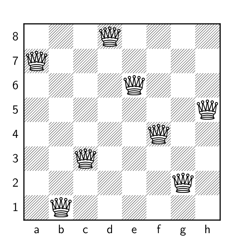
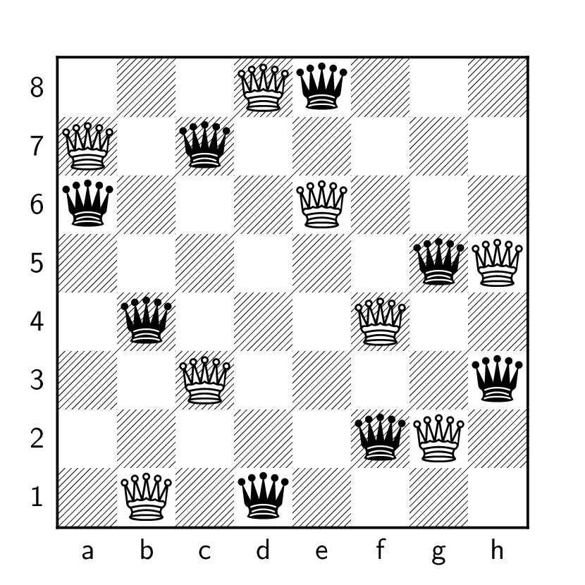
consider. One of them is shown in Figure 18.1(a); can you
find a different solution yourself?
We can keep going. Figure 18.1(b) shows
two simultaneous solutions to the \(8\)
queens puzzle that do not share any squares: one with \(8\) white queens, and one with \(8\) black queens. An even more impressive
solution was found by Rob Pratt [85], who placed six solutions to the \(8\) queens puzzle on a chessboard
simultaneously, and verified that more is impossible.
In fact, without seeing either of the
diagrams in Figure 18.1,
you can argue that if a solution to the \(8\) queens puzzle exists, then we can solve
the version with \(16\) queens as well.
How?
Combine a solution to the \(8\) queens puzzle with its mirror image!
The mirror image of a queen’s location cannot be occupied by another
queen, because then those two queens would attack each other.
Both of these problems can be modeled using graph theory. For the
\(8\) queens puzzle itself, we define
the \(8\times 8\) queen graph
to have \(64\) vertices, one for each
square of the chessboard, with an edge for between every two vertices
that share a rank, file, or diagonal. Then our goal is to select \(8\) vertices from this graph with no edges
between them.
For the problem of simultaneous solutions in multiple colors, define
a graph whose \(92\) vertices are the
\(92\) different possible solutions to
the \(8\) queens puzzle, Make two
vertices adjacent if the solutions overlap, so that they cannot be
placed on the chessboard simultaneously. Then our goal is to select as
many vertices as possible from this graph with no edges between
them—another instance of the same problem!
In general, we make the following definitions:
Definition 18.1. An independent
set in a graph \(G\) is a set
of vertices \(I \subseteq V(G)\) such
that no two vertices in \(I\) are
adjacent. The independence number of \(G\), denoted \(\alpha(G)\), is the number of vertices in a
maximum independent set in \(G\).
We defined the graphs in our previous problems such that edges
represent conflicts, and so the set that we want to choose is a set of
vertices with no edges between them. Instead, we could have defined the
graphs so that edges represent compatibility. That is, two squares on
the chessboard would be adjacent if two queens on those squares do not
attack each other, and two solutions to the \(8\) queens puzzle would be adjacent if they
do not overlap. This graph would be the complement of the \(8\times 8\) queen graph.
If we had done this, we would be looking for a different object,
which has its own definition.
Definition 18.2. A clique in a
graph \(G\) is a set of vertices \(Q \subseteq V(G)\) such that every pair of
vertices in \(Q\) is adjacent. The
clique number of \(G\), denoted \(\omega(G)\), is the number of vertices in a
maximum clique in \(G\).
It is hard to say why \(\alpha\)
(alpha) and \(\omega\) (omega) were
chosen to represent these quantities, but at the very least there is
some relationship there: \(\alpha\) is
the first letter in the Greek alphabet, and \(\omega\) is the last.
Previously, we’ve referred to complete graphs as cliques, and this is
not a coincidence: a set of vertices \(Q\) is a clique precisely when the induced
subgraph \(G[Q]\) is a copy of the
complete graph \(K_{|Q|}\). In
principle, we could have defined cliques to be complete subgraphs of
\(G\), but this is not as useful. The
edges in the subgraph don’t tell us anything: they are simply all
present.
What kind of subgraph is induced by a
\(m\)-vertex independent set?
A copy of \(\overline{K_m}\), also known as the empty
graph.
The queen graph is a bit asymmetric: the corner and edge vertices
have fewer neighbors. A more mathematically elegant version of the
problem makes all vertices equal, by allowing queen moves that wrap
around the board. For example, the diagonal through the squares f1, g2, h3 would continue to a4, b5, and so
on, as though we had glued opposite sides of the board to make a
cylinder.
More generally, we define the periodic \(n\times n\) queen graph to have vertices
\((x,y)\) where \(1 \le x \le n\) and \(1 \le y \le n\); here, \(x\) and \(y\) represent the horizontal and vertical
coordinates of a square. Two vertices \((x_1,
y_1)\) and \((x_2, y_2)\) are
adjacent when \(x_1 = x_2\) or \(y_1 = y_2\) or \(x_1 + y_1 \equiv x_2 + y_2 \pmod n\) or
\(x_1 - y_1 \equiv x_2 - y_2 \pmod n\).
The “mod \(n\)” is what makes the board
wrap around. With this modification, the side and corner squares are now
just like every other square of the board.
Unfortunately, there is no \(8\)-vertex independent set in the periodic
\(8\times 8\) queen graph: no solution
to the \(8\) queens problem on a board
that wraps around. George Pólya proved this in 1921 [82], along with a general
statement: the periodic \(n \times n\)
queen graph has an \(n\)-vertex
independent set exactly when \(n\) is
not divisible by \(2\) or \(3\).
Remarkably, in such cases, we can even place \(n\) disjoint solutions on the \(n\times n\) board, occupying every square!
This object is known as a Knut Vik design, and has applications in
minimizing the variability of statistical experiments. A Knut Vik design
for all \(n \times n\) boards where
\(n\) is not divisible by \(2\) or \(3\) was first constructed by Samad Hedayat
and Walter Federer in 1975 [55].
(In general, a partition of a graph into independent sets is called a
proper coloring, and will be discussed in the next
chapter.)
Redundancies and
relationships
Applications such as the \(8\)
queens puzzle could be modeled either by cliques or by independent sets.
Why, then, do we define both invariants to begin with? We could simply
adopt the convention that we always use the “conflict” definition, where
two vertices are adjacent if they’re incompatible. Then, we’d always be
looking for independent sets, and we’d never need to know the definition
of a clique.
We can always reduce the problem of
finding cliques in a graph \(G\) to
finding independent sets, even if it did not arise from such an
application. How?
Take the complement graph \(\overline G\), which has exactly the edges
not present in \(G\). Then a clique in
\(G\) is precisely an independent set
in \(\overline G\).
One of the reasons we don’t do this is that we might prefer one
version of the graph for other reasons. This is true of the \(8\times 8\) queen graph where two vertices
are adjacent if a queen on one square attacks the other, for example. In
this graph, walks correspond to possible sequences of queen moves, which
could have other applications. So if we want to keep the same definition
of the graph for multiple puzzles, this forces our hand.
Sometimes it is even interesting to study both cliques and
independent sets in the same graph. For example, this occurs in some
scheduling problems. If we are scheduling a number of events (such as
presentations at a conference or a convention) then we might want to
think about which events are happening at the same time: we could make a
graph where every event is a vertex, and two vertices are adjacent if
the event times overlap.
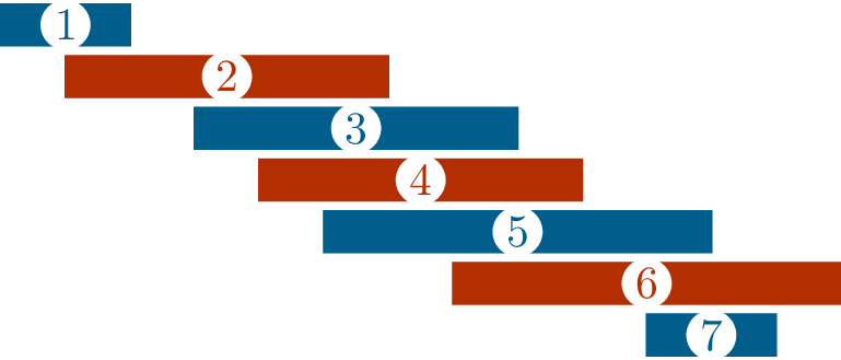
Slightly more generally, suppose we have a set of intervals \[[a_1, b_1], [a_2, b_2], \dots, [a_n,
b_n]\] in the real line. (In the scheduling problem, \(a_i\) and \(b_i\) are the starting and ending time of
the \(i\)th event.) Then we
can define a graph whose vertices are these intervals, with an edge
whenever two intervals overlap. Such a graph is called an
interval graph.1
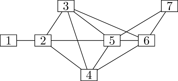
Figure 18.2 shows a collection of
intervals, together with the corresponding interval graph.
In an interval graph representing a
schedule of events, what would a clique represent?
A clique corresponds to a set of intervals
that all overlap: a set of events all happening at the same time. (You
might care, for example, because you want to put them all in different
rooms.)
What would an independent set
represent?
An independent set corresponds to a set of
disjoint intervals: a set of events that don’t conflict. (You might
care, for example, because you want to attend all of them.)
Returning to the original topic, another reason to study both cliques
and independent sets is that we might study the relationship between
these objects and other properties of the graph. For example, we might
ask: how does the maximum degree of a graph affect the clique number,
and how does it affect the independence number? Both are valid
questions, with very different answers.
In fact, there are already such connections to be explored. The
independence number \(\alpha(G)\) is
closely related to both invariants introduced in Chapter 14: the matching number \(\alpha'(G)\) and the vertex cover
number \(\beta(G)\).
As far as the matching number goes, you might be a bit suspicious due
to the similar notation. It is not an accident: the \('\) symbol indicates that \(\alpha'(G)\) is the “edge version” of
\(\alpha(G)\). Where \(\alpha(G)\) is the maximum number of
vertices that do not share any edge, \(\alpha'(G)\) is the maximum number of
edges that do not share any vertex. We will explore this connection and
others like it in more detail in Chapter 20.
It is the connection to \(\beta(G)\)
that you might be surprised by.
Suppose \(U\) is a particularly small vertex cover in
a graph \(G\): a set of vertices
including at least one endpoint of every edge. How can we use it to find
a particularly large independent set in \(G\)?
The set \(I =
V(G) - U\) consisting of all vertices not in \(U\) is an independent set!2 If
two vertices \(x,y \in I\) were
adjacent, then \(U\) would not contain
any endpoint of the edge \(xy\),
contradicting its status as a vertex cover.
Numerically: \(\alpha(G) = |V(G)| -
\beta(G)\). Once again, the question arises: why do we have two
invariants \(\alpha(G)\) and \(\beta(G)\) when one of them can easily be
used to obtain the other?
A good answer in this particular case is that we might be interested
in ratios between the number of vertices in two independent sets, or two
vertex covers. For example, if we have an algorithm that finds a vertex
cover of at most \(2\beta(G)\)
vertices, or an independent set of at least \(\frac12 \alpha(G)\) vertices, we might say:
that’s within a factor of \(2\) of the
true answer, so the guarantee is good enough.
In fact, such an approximation algorithm for vertex covers does
exist—but such an approximation algorithm for independent sets does not,
as far as we know! That’s because the relationship \(I = V(G) - U\) does not play well with
ratios: doubling the size of the set \(U\) is not at all the same thing as halving
the size of the set \(I\).
Greedy algorithms
In general, algorithms that find maximum cliques or maximum
independent sets must do so by backtracking: pick a vertex, try
including it, and if it doesn’t work out, try leaving it out. This is
better than trying all \(2^{|V(G)|}\)
sets of vertices one by one: if we pick a vertex, then we can make some
deductions about which other vertices cannot be picked. However, even
the best backtracking algorithms take an exponentially long time to
finish.
If we want an answer quickly, we must give up on insisting that we
get the right answer. The most basic technique is to use a greedy
algorithm: to pick vertices to add to our set without considering the
consequences for future decisions, and to see where that gets us.
Here is one possible greedy algorithm for finding an independent set
\(I\) in a graph \(G\). We begin by setting \(I = \varnothing\); we also keep track of a
set \(A\) which contains all the
vertices that are still available for use. Initially, \(A = V(G)\). A single iteration of the
greedy algorithm consists of the following steps:
Let \(x\) be any vertex in \(A\); add it to the independent set,
replacing \(I\) by \(I \cup \{x\}\).
Replace \(A\) by \(A - (\{x\} \cup N(\{x\}))\): remove both
\(x\) and \(N(\{x\})\) (the set of vertices adjacent to
\(x\)) from \(A\).
If \(A = \varnothing\),
stop.
It is impossible for the set \(I\)
to ever contain two adjacent vertices \(x\) and \(y\): if we ever add \(x\) to \(I\), we remove \(y\) from \(A\), and if we ever add \(y\) to \(I\), we remove \(x\) from \(A\). Therefore the output of this algorithm
is guaranteed to be an independent set.
If we want a greedy algorithm for finding
a clique, how should we modify this algorithm?
At each iteration, we should replace \(A\) by \(A \cap
N(\{x\})\) instead, so that all vertices we add in future
iterations are adjacent to \(x\).
What’s more, the output \(I\) is
guaranteed to be a maximal independent set (following the
maximal/maximum distinction introduced in Chapter 13). The set \(I\) is not necessarily the largest
independent set, but there is no bigger independent set \(I'\) that contains all of \(I\). This is true because every vertex
\(y \in V(G)\) is removed from \(A\) in some iteration, for one of two
reasons:
\(y\) is equal to \(x\), the vertex added to \(I\) in that iteration.
\(y\) is adjacent to \(x\).
In both cases, \(I \cup \{y\}\) is
not a bigger independent set. In the first case, that’s because \(I \cup \{y\}\) is the same set as \(I\). In the second case, that’s because
\(I \cup \{y\}\) is not an independent
set; it contains the edge \(xy\).
This proves that \(I\) is a maximal
independent set. However, \(I\) is not
guaranteed to be a maximum independent set: there may well be other
independent sets which are larger.
Can you find a graph in which the set
\(I\) we find is much smaller than
another independent set?
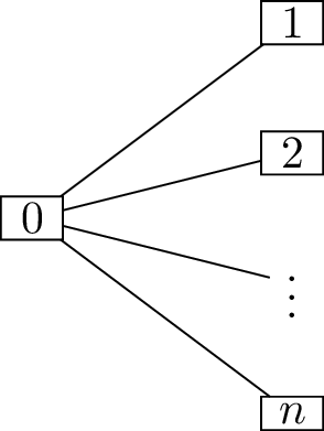
One of many examples is the graph shown in
Figure 18.3(a): a copy of the star graph \(S_{n+1}\). If the algorithm adds vertex
\(0\) to \(I\), it will immediately get \(A = \varnothing\) and stop; however, \(I = \{0\}\) is much smaller than the
independent set \(\{1,2,3,\dots,n\}\).
We might say: okay, the problem is clear. We chose a vertex with very
high degree and removed all its neighbors from \(A\), causing the algorithm to stop very
quickly. What if we try to be smarter about step 1 of the algorithm, so
that at each iteration we choose the vertex \(x\) with the fewest neighbors in \(A\)?
This might sometimes be a useful heuristic, but it is not guaranteed
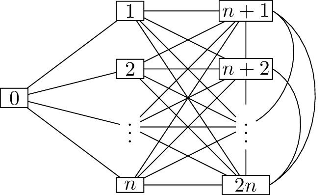
to work. Consider instead the graph in Figure 18.3(b); here, we’ve added
vertices \(n+1, n+2, \dots, 2n\),
adjacent to vertices \(1, 2, \dots, n\)
and to each other.
A star graphExtending the star graph
Graphs which confuse the greedy independent set
algorithmWhat will the greedy algorithm do, given
the graph in Figure 18.3(b),
if it chooses the vertex with the fewest neighbors in \(A\) at each step?
The first vertex chosen will still be
vertex \(0\), because it has degree
\(n\) and all other vertices have
degree at least \(n+1\). Then, vertices
\(1, \dots, n\) will be deleted, and
the second vertex will be one of \(n+1, \dots,
2n\). Then, all remaining vertices will be deleted, and the
algorithm will find a \(2\)-vertex
independent set.
What is the largest independent set in the
graph in Figure 18.3(b)?
The set \(\{1,2,\dots,n\}\), which is \(\frac{n}{2}\) times bigger than the set
found by the greedy algorithm.
There is no rule for choosing vertices in the greedy algorithm that’s
always guaranteed to do well. However, at the very least, we can use the
greedy algorithm to prove worst-case bounds.
Proposition 18.1. If \(G\) is an \(n\)-vertex graph with maximum degree \(\Delta(G)\), then \(\alpha(G) \ge
\frac{n}{\Delta(G)+1}\).
Proof. To prove the lower bound, we find an independent set
in \(G\) using the greedy algorithm,
taking no special care in choosing the vertex \(x\) at each iteration.
Nevertheless, what we can guarantee is that at each iteration, at
most \(\Delta(G) + 1\) vertices are
removed from \(A\). We remove \(x\) and all neighbors of the chosen vertex
\(x\) in \(A\). There are at most \(\Delta(G)\) such neighbors; there could be
fewer if \(\deg_G(x) < \Delta(G)\),
or if not all neighbors of \(x\) are
still in \(A\), but there cannot be
more.
The algorithm does not stop until \(A\) is empty, but since each iteration
removes at most \(\Delta(G)+1\) out of
\(n\) vertices from \(A\), there must be at least \(\frac{n}{\Delta(G)+1}\) iterations. At each
iteration, one vertex is added to \(I\); therefore, the output of the algorithm
is an independent set \(I\) with at
least \(\frac{n}{\Delta(G)+1}\)
vertices. Therefore \(\alpha(G)\) is
also at least \(\frac{n}{\Delta(G)+1}\). ◻
What lower bound can we get for the clique
number \(\omega(G)\)?
Since \(\omega(G) = \alpha(\overline{G})\), we have
\[\omega(G) \ge \frac{n}{\Delta(\overline G)
+ 1} = \frac{n}{n - \delta(G)},\] where \(\delta(G)\) is the minimum degree of \(G\).
Here, the identity \(\Delta(\overline G) =
n-1 -\delta(G)\) holds because a maximum-degree vertex in \(\overline G\) is a minimum-degree vertex in
\(G\), and because \(\deg_{\overline G}(x) = n-1-\deg_G(x)\) for
any vertex \(x\).
An indecisive algorithm
In preparation for our next topic, consider a variant of the greedy
algorithm that hasn’t made up its mind yet about whether it wants to
find a clique or an independent set. It will still keep track of a set
\(A\) of available vertices, initially
equal to \(V(G)\). It will also build
up a set we’ll simply call \(S\),
initially equal to \(\varnothing\); at
each iteration, it will move a vertex \(x\) from \(A\) to \(S\), then update \(A\).
The upside to being indecisive is that at each iteration, the
algorithm has a choice:
It could remove \(x\) and all of
its neighbors from \(A\).
It could remove \(x\) and all
vertices which are not its neighbors from \(A\).
If the algorithm always chooses the option that keeps \(A\) as large as possible, then it’s
guaranteed to keep at least \(\frac{|A|-1}{2}\) vertices for the next
iteration (rounded up). It must always remove \(x\), but it can keep at least half of the
remaining vertices.
The downside to being indecisive is that the final set \(S\) will not be either a clique or an
independent set. Suppose that after \(k\) iterations, we obtain \(S = \{x_1, x_2, \dots, x_k\}\), where \(x_i\) is the vertex added to \(S\) at the \(i\)th iteration.
Is there any useful property at all that
this set \(S\) has?
We can at least guarantee that a vertex
\(x_i\) is either adjacent to all of
the vertices \(x_{i+1}, x_{i+2}, \dots,
x_k\), or to none of them. The first case occurs when we removed
all the non-neighbors of \(x_i\) from
\(A\) in the \(i\)th iteration; the second case
occurs when we removed all the neighbors of \(x_i\) from \(A\) in the \(i\)th iteration.
This property seems hard to make use of, but let’s try. Suppose we
call a vertex \(x_i\) a “Q-type” vertex
(Q for clique) if it is adjacent to all of \(x_{i+1}, x_{i+2}, \dots, x_k\), and a
“I-type” vertex (I for independent set) if it is adjacent to none of
these vertices. We can write \(S\) as
the union \(Q \cup I\), where \(Q\) is the set of all Q-type vertices and
\(I\) is the set of all I-type
vertices.
What can we say about \(Q\) and \(I\)?
\(Q\) is
a clique and \(I\) is an independent
set.
What is the type of vertex \(x_k\)?
It is both Q-type and I-type, since there
are no vertices that come after it, so both conditions are vacuously
true.
Except for \(x_k\), every vertex is
only one of Q-type or I-type, so \(|Q| + |I| =
|S|+1\). Therefore, if the indecisive algorithm only picks at the
last possible moment whether to return the clique \(Q\) or the independent set \(I\), it is guaranteed to find a set of
\(\frac{|S|+1}{2}\) vertices.
The indecisive algorithm is not usually useful in practice: for most
problems, we have already decided whether we are looking for a clique or
an independent set. However, we can use it to prove a relationship
between these quantities.
Proposition 18.2. If \(G\) is a graph with at least \(2^{n-2}\) vertices, then \(\alpha(G) + \omega(G) \ge n\). In other
words, \(\alpha(G) + \omega(G) \ge 2 + \log_2
|V(G)|\).
Proof. Apply the indecisive algorithm to \(G\). At the beginning, \(|A| \ge 2^{n-2}\). After one iteration, we
replace \(A\) by a set with at least
\(\frac{|A|-1}{2}\) elements in it, so
we can say that \(|A| \ge
\frac{2^{n-2}-1}{2}\); rounding up, \(|A| \ge 2^{n-3}\). Similarly, after a
second iteration, we can still guarantee \(|A|
\ge 2^{n-4}\). This argument can be repeated for as long as our
lower bound on \(|A|\) is even,
ensuring that \(\frac{|A|-1}{2}\) can
be rounded up to \(\frac{|A|}{2}\).
After the \((n-2)\)th
iteration, we can guarantee that \(|A| \ge
2^{n-(n-2)-2}\), or \(|A| \ge
1\). This is still enough to know that there will be an \((n-1)\)th iteration. However,
it’s possible that the \((n-1)\)th iteration is the last,
because it removes the only remaining element in \(A\).
At the end, the indecisive algorithm chooses between returning a
clique \(Q\) or an independent set
\(I\), which satisfy \(|Q| + |I| = |S|+1\). Since \(|S| \ge n-1\), we conclude that \(|Q| + |I| \ge n\). This completes the
proof, since \(\alpha(G)\) is at least
\(|I|\) and \(\omega(G)\) is at least \(|Q|\): the largest clique and independent
set are at least as large as the ones we found. ◻
Intuitively, we can make the independence number \(\alpha(G)\) small by giving \(G\) lots of edges, and we can make the
clique number \(\omega(G)\) small by
giving \(G\) few edges. However, these
strategies directly oppose each other, so it makes sense that we
wouldn’t be able to keep both \(\alpha(G)\) and \(\omega(G)\) from growing. Proposition 18.2 is the first result we will
prove that quantifies this relationship.
Ramsey numbers
We can improve on Proposition 18.2 by
noticing a flaw in how the indecisive algorithm chooses which vertices
to keep in \(A\). All it does is pick
the option that keeps \(A\) as large as
possible, but if you want the final clique or independent set to be as
large as possible, that’s not always correct.
Why would you ever decide to keep a
smaller set to be set \(A\) in the next
iteration?
Suppose that the current set \(S\) contains many Q-type vertices and few
I-type vertices. Then you might keep all the neighbors of \(x\) in \(A\), making \(x\) another Q-type vertex, even if the
algorithm stops a bit sooner as a result.
To be strategic about it, we need to quantify the exact trade-off:
how many fewer vertices in \(A\) are an
acceptable price to pay in exchange for guaranteeing a vertex of the
right type? This depends on our goals, of course. If we’d be happy with
a clique of size \(100\) and we already
have \(98\) Q-type vertices, we should
make \(x\) another Q-type vertex at
almost any cost—even if \(x\) only has
one or two neighbors in \(A\). If we’re
further from our goal, we should be more conservative.
That’s still vague; to make it more concrete, we need to know exactly
how many vertices in \(A\) are
necessary to reach any particular goal we might have. So for integers
\(k\ge 1\) and \(l \ge 1\), we define the Ramsey
number\(R(k,l)\) to be the least
integer \(n\) such that any \(n\)-vertex graph \(G\) satisfies either \(\alpha(G) \ge k\) or \(\omega(G) \ge l\).
Can we be certain that any such integer
\(n\) exists?
Yes, by Proposition 18.2. Take a graph \(G\) with \(n =
2^{k+l-3}\) vertices; then \(\alpha(G)
+ \omega(G) \ge k+l-1\), which cannot be true if both \(\alpha(G) \le k-1\) and \(\omega(G) \le l-1\). Therefore \(2^{k+l-3}\) vertices are enough, and \(R(k,l)\) is at most this big.
Ramsey numbers are named after Frank Ramsey, who was the first to
prove a result analogous to Proposition 18.2 in
1930 [89], though he was
not interested in concrete bounds on the necessary number of
vertices.
Let me describe a concrete situation to motivate our need for Ramsey
numbers. Suppose we are looking for a clique or an independent set of
size \(5\). Currently, we have \(3\) vertices in \(S\): two Q-type vertices (adjacent to each
other and all vertices in \(A\)) and
one I-type vertex (with no neighbors in \(A\)). We’ve chosen a vertex \(x\) in the fourth iteration, and we’re
considering what to do with the neighbors of \(x\) to prepare for the next iteration.
If we keep all the neighbors of \(x\) in \(A\), then \(x\) will be another Q-type vertex. We will
need to find either two more Q-type vertices or four more I-type
vertices in the future.
If we keep all the non-neighbors of \(x\) in \(A\), then \(x\) will be another I-type vertex. We will
need to find either three more Q-type vertices or three more I-type
vertices in the future.
How should we choose between these two
options?
If \(x\)
has at least \(R(4,2)\) neighbors in
\(A\), then the first option is
guaranteed to succeed. If \(x\) has at
least \(R(3,3)\) non-neighbors in \(A\), then the second option is guaranteed
to succeed. If neither is true, then both options are risky, and we
might need to guess.
Some people are very comfortable with algorithms; some people prefer
more mathematical arguments. In case you are the second type of person,
you will be happier with the following lemma, whose proof is inspired by
the indecisive algorithm but doesn’t use it directly.
Lemma 18.3. For all integers \(k\ge 2\) and \(l\ge 2\), the Ramsey number \(R(k,l)\) is at most the sum \(R(k,l-1) + R(k-1,l)\).
Proof. Let \(G\) be an
arbitrary graph with \(R(k-1,l) +
R(k,l-1)\) vertices. Our goal is to prove that this is enough to
guarantee that either \(\alpha(G) \ge
k\) or \(\omega(G) \ge l\).
Choose any vertex \(x \in V(G)\),
and divide \(V(G) - \{x\}\) into two
sets: \(A_1\), the vertices adjacent to
\(x\), and \(A_2\), the vertices not adjacent to \(x\).
It is impossible that both \(|A_1| <
R(k,l-1)\) and that \(|A_2| <
R(k-1,l)\). In that case, \(|V(G)| =
|A_1| + |A_2| + 1\) would be at most \((R(k,l-1) - 1) + (R(k-1,l) - 1) + 1\) or
\(R(k-1,l) + R(k,l-1) - 1\): one less
than the number of vertices we defined \(G\) to have.
If \(|A_1| \ge R(k,l-1)\), then the
induced subgraph \(G[A_1]\) is big
enough to either contain a \(k\)-vertex
independent set \(I\) or an \((l-1)\)-vertex clique \(Q\), by the definition of the Ramsey number
\(R(k,l-1)\). Therefore \(G\) contains either a \(k\)-vertex independent set \(I\) or an \(l\)-vertex clique \(Q \cup \{x\}\) (since \(x\) is adjacent to all vertices in \(A_1\), and in particular all vertices in
\(Q\)).
If instead \(|A_2| \ge R(k-1,l)\),
then \(G[A_2]\) is big enough to either
contain a \((k-1)\)-vertex independent
set \(I\) or an \(l\)-vertex clique \(Q\). Therefore \(G\) contains either a \(k\)-vertex independent set \(I \cup \{x\}\) or an \(l\)-vertex clique \(Q\).
In all cases, we either find a \(k\)-vertex independent set or and \(l\)-vertex clique in \(G\). Since \(G\) was chosen to be an arbitrary graph
with \(R(k-1,l) + R(k,l-1)\) vertices,
this proves that \(R(k,l) \le R(k-1,l) +
R(k,l-1)\). ◻
Lemma 18.3 is the foundation of a
recurrence that can be used to get upper bounds on the Ramsey numbers.
To use the recurrence, we also need base cases.
Lemma 18.3 starts at \(k\ge 2\) and \(l\ge 2\). What is \(R(k,l)\) when \(k=1\) or when \(l=1\)?
In all these cases, it is just \(1\); even something like \(R(1,10000)\) is \(1\). There is only one possible \(1\)-vertex graph, and it has both a \(1\)-vertex clique and a \(1\)-vertex independent set.
\(R(k,2)\) and \(R(2,l)\) can also be computed exactly; what
are they?
\(R(k,2)=k\) and \(R(2,l)=l\). For the first of these, suppose
we have a \(k\)-vertex graph. Either it
has no edges (and there is a \(k\)-vertex independent set) or it has an
edge \(xy\) (and \(\{x,y\}\) is a \(2\)-vertex clique). The argument for \(R(2,l)\) is similar.
The general upper bound on \(R(k,l)\) using this recurrence is sometimes
also called Ramsey’s theorem, but actually, it was only proven in 1955
by Robert Greenwood and Andrew Gleason [40] (who also proved Lemma 18.3 in the process).
Theorem 18.4. For all integers \(k \ge 1\) and \(l\ge 1\), \(R(k,l) \le \binom{k+l-2}{k-1}\).
Proof. We induct on \(k+l\). (That is, if \(P(n)\) is the statement that the theorem
holds for all integers \(k\ge 1\) and
\(l\ge 1\) with \(k+l=n\), then we prove \(P(n)\) for all \(n\ge 1\) by induction on \(n\).)
As our base case, we can take any of \(k+l=1\) (where there is nothing to prove),
or \(k+l=2\) (where \(R(1,1) = 1 = \binom 00\)), or \(k+l=3\) (where \(R(2,1) = 1 = \binom 10\) and \(R(1,2) = 1 = \binom11\)), but eventually we
will have to induct.
Consider some \(k \ge 1\) and \(l\ge 1\) with \(k+l \ge 3\), and assume the following
induction hypothesis: for all \(k'\ge
1\) and \(l' \ge 1\) with
\(k'+l' = k+l-1\), we have the
upper bound \(R(k', l') \le
\binom{k'+l'-2}{k'-1}\). Actually, we only need it
for two values of \(k'\) and \(l'\): the ones that appear in the
right-hand side of Lemma 18.3.
If \(k=1\) or \(l=1\), we cannot apply Lemma 18.3; what do we do?
If \(k=1\) or \(l=1\), we know that \(R(k,l)=1\), and in both cases the upper
bound \(\binom{k+l-2}{k-1}\) simplifies
to \(\binom{l-1}0 = 1\) or \(\binom{k-1}{k-1} = 1\), so we do not even
need the induction hypothesis.
Otherwise, \(k\ge 2\) and \(l\ge 2\). By Lemma 18.3, \(R(k,l) \le R(k,l-1) + R(k-1,l)\), and both
of the Ramsey numbers on the right-hand side are suitable for the
induction hypothesis. We can conclude that \[R(k,l) \le \binom{k+(l-1)-2}{k-1} +
\binom{(k-1)+l-2}{(k-1)-1} = \binom{k+l-3}{k-1} +
\binom{k+l-3}{k-2}.\] The right-hand side of this inequality
simplifies directly to \(\binom{k+l-2}{k-1}\). This is called
Pascal’s identity, and if you haven’t seen it before, there is a short
combinatorial argument. By its combinatorial definition, \(\binom{k+l-2}{k-1}\) counts the \((k-1)\)-element subsets \(S \subseteq \{1,2,\dots,k+l-2\}\). These
come in two types. If \(k+l-2 \notin
S\), then \(S\) is a subset of
\(\{1,2,\dots,k+l-3\}\), and so there
are \(\binom{k+l-3}{k-1}\) cases of
this type. If \(k+l-2 \notin S\), then
\(S - \{k+l-2\}\) is a \((k-2)\)-element subset of \(\{1,2,\dots,k+l-3\}\), and so there are
\(\binom{k+l-3}{k-2}\) cases of this
type.
Altogether, there must be \(\binom{k+l-3}{k-1} + \binom{k+l-3}{k-2}\)
subsets. We already know there are \(\binom{k+l-2}{k-1}\) subsets, so these two
expressions must be equal. Returning to our upper bound on \(R(k,l)\), we can replace one expression by
the other and get \(R(k,l) \le
\binom{k+l-2}{k-1}\). This proves the induction step, completing
the proof of the theorem. ◻
Both Ramsey and later Greenwood and Gleason also considered a
generalized problem. Here, we define the Ramsey number \(R(k_1, k_2, \dots, k_m)\) to be the least
\(n\) with the following property:
whenever we write the complete graph \(K_n\) as the union of \(n\)-vertex graphs \(G_1 \cup G_2 \cup \dots \cup G_m\), there
will be some \(G_i\) such that \(\omega(G_i) \ge k_i\). Sometimes, this is
phrased as coloring the edges of \(K_n\) using \(m\) different colors, but I will avoid this
so that you don’t confuse it with all the other ways we will color a
graph.
Lower bounds
Once we have defined Ramsey numbers, it is tempting to try to figure
out an exact formula for them, or at least an approximate one. Our first
upper bound on \(R(k,l)\) was \(2^{k+l-3}\), and our second bound of \(\binom{k+l-2}{k-1}\) has a similar rate of
growth, at least when \(k=l\). Is this
anywhere close to the truth? How would we know?
In the definition of the Ramsey number \(R(k,l)\), we ask for the least \(n\) such that every \(n\)-vertex graph satisfies a condition. To
prove that \(R(k,l) \ge n\), it is
enough to find a single \((n-1)\)-vertex graph which does not yet
satisfy the condition. (Such graphs are sometimes called Ramsey graphs,
because of their use in proving lower bounds for Ramsey numbers.)
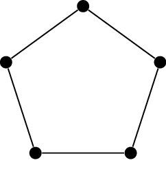
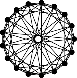
The cycle graph \(C_5\)\(\operatorname{Ci}_8(1,4)\)\(\operatorname{Ci}_{17}(1,2,4,8)\)
The cycle graph \(C_5\), shown
in Figure 18.4(a), has no \(3\)-vertex clique or \(3\)-vertex independent set. This proves
that \(R(3,3) \ge 6\): we need at least
\(6\) vertices to guarantee one of
these objects, because \(5\) are not
enough.
In fact, Theorem 18.4 proves an upper bound of \(\binom{3+3-2}{3-1} = \binom 42 = 6\) on
\(R(3,3)\), so we know that \(R(3,3)=6\).
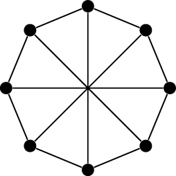
The circulant graph \(\operatorname{Ci}_8(1,4)\) shown in
Figure 18.4(b) has no \(3\)-vertex clique or \(4\)-vertex independent set, and it has
\(8\) vertices, so it proves that \(R(4,3) \ge 9\). Theorem 18.4 only proves that \(R(4,3) \le \binom{4+3-2}{4-1} = \binom 53 =
10\), but in one of the practice problems, I will ask you to
improve this upper bound: in fact, \(R(4,3)=9\).
What about \(R(3,4)\)?
It is also equal to \(9\); in fact, \(R(k,l)\) and \(R(l,k)\) are always equal. The lower bound
that proves \(R(3,4)\ge 9\) is the
complement of \(\operatorname{Ci}_8(1,4)\): the circulant
graph \(\operatorname{Ci}_8(2,3)\). A
similar trick of complements can be used to show that every \(n\)-vertex graph contains a \(k\)-vertex independent set or an \(l\)-vertex clique, then it is also true
that every \(n\)-vertex graph contains
an \(l\)-vertex independent set or a
\(k\)-vertex clique.
Taking \(R(3,4) = R(4,3)=9\) for
granted, it follows from Lemma 18.3 that \(R(4,4) \le R(4,3) + R(3,4) = 18\). In fact,
\(R(4,4) = 18\); to prove this, we need
a \(17\)-vertex graph.
The graph in Figure 18.4(c) is one
such graph: the circulant graph \(\operatorname{Ci}_{17}(1,2,4,8)\). This
graph has no \(4\)-vertex clique or
\(4\)-vertex independent set, so it
proves the lower bound \(R(4,4) \ge
18\).
Of course, we cannot go on forever like this; to give a general lower
bound, some general scheme for constructing these graphs is needed.
Unfortunately, it has been very difficult to construct these graphs. We
run into two kinds of problems. First, most simple rules defining an
arbitrarily large graph will give it a large clique or a large
independent set. Second, when we eventually do find a general
construction that looks promising, we often find out that proving
something about its cliques or independent sets turns into an unsolved
problem in number theory.
(Why number theory? Well, the offsets of the circulant graph \(\operatorname{Ci}_{17}(1,2,4,8)\) in
Figure 18.4(c) are not arbitrary: they are the
quadratic residues modulo \(17\). That
is, every perfect square is congruent modulo \(17\) to one of \(\pm 1\), \(\pm
2\), \(\pm 4\), or \(\pm 8\). Graphs constructed in this way are
called Paley graphs, and they are often useful for proving lower bounds
on Ramsey numbers; however, we don’t understand quadratic residues well
enough to say what the lower bounds are in general.)
The best we’ve been able to do is to give up and pick a graph at
random, showing that the result is very unlikely to have a large clique
or a large independent set. Let me first illustrate this with concrete
numbers. Suppose we define a graph \(G\) on \(1 000
000\) vertices by flipping a coin for every possible edge to see
if it’s present or absent. What are the odds that this random graph
\(G\) will have a \(40\)-vertex clique?
There are \(\binom{1 000 000}{40} \approx
1.22 \times 10^{192}\) ways to choose \(40\) of the vertices of \(G\). Each one of those \(40\)-vertex sets could in theory be a \(40\)-vertex clique… but that’s very
unlikely. There are \(\binom{40}{2} =
780\) edges between those \(40\)
vertices, so we flip \(780\) coins to
decide which edges between the vertices are present. In order for us to
get a clique, all the coin flips have to go one way, which has a
probability of \(2^{-780} \approx 1.57 \times
10^{-235}\).
If you bought \(\binom{1 000
000}{40}\) tickets for a lottery that chose one winning ticket
out of \(2^{780}\), then to find your
total chances of winning, it would be enough to multiply these two
numbers together. This would give us \((1.22
\times 10^{192}) \cdot (1.57 \times 10^{-235})\) or about \(1.93 \times 10^{-43}\). The clique problem
is actually even worse, due to overlaps. After we consider the first
clique, the second doesn’t contribute its whole \(2^{-780}\) probability, because some of
those cases were already counted: the two cliques appear
simultaneously!
Rather than consider what the situation with overlaps is, we can
simply say that the probability of having a \(40\)-vertex clique is at most \(1.93 \times 10^{-43}\). We get the same
probability for a \(40\)-vertex
independent set: once again, all the coin flips have to go one way for
all \(780\) edges between vertices of a
set. Since both probabilities are tiny, we conclude that this random
\(1000000\)-vertex graph is almost
certain not to have a \(40\)-vertex
clique or \(40\)-vertex independent
set, proving that \(R(40,40) >
1000000\).
In 1947, Pál Erdős proved [28] that this gives an exponential lower bound
on the Ramsey numbers:
Theorem 18.5. For all \(k \ge 3\), \(R(k,k) > 2^{k/2}\).
Proof. Pick a random graph on \(n
= 2^{k/2}\) vertices by flipping a coin for every edge. There are
\(\binom nk\) possible \(k\)-vertex sets; each has a \(2^{-\binom k2}\) chance of being a clique,
and another \(2^{-\binom k2}\) chance
of being an independent set, for a total probability of \(2^{1-\binom k2}\) of doing anything of
interest.
As before, we get an upper bound on the probability that any of these
cliques or independent sets are created by multiplying these quantities
together: \(\binom nk \cdot 2^{1-\binom
k2}\). It is always true that \(\binom
nk \le \frac{n^k}{k!}\), and for \(k\ge
3\), it is true that \(k! >
2^k\). Applying both inequalities, our upper bound becomes \(n^k \cdot 2^{-k} \cdot 2^{1 - k^2/2 +
k/2}\) or \(2^{1-k/2}\), which
is less than \(1\) as soon as \(k\ge 3\).
Therefore the probability that the random graph doesn’t do what we
want is less than \(1\): some of the
\(n\)-vertex graphs we could get have
neither \(k\)-vertex cliques nor \(k\)-vertex independent sets. This shows
that \(R(k,k) > n\). ◻
The bounds \(R(k,k) > 2^{k/2}\)
and \(R(k,k) \le \binom{2k-2}{k-1}\)
(which grows roughly as \(2^{2k}\)) are
fairly far apart, though they are both exponential; for example, they
tell us that \(32 < R(10,10) \le
48620\). It has been at least 70 years since any of the results
mentioned in this chapter so far; has there been improvement since
then?
There has been and there still is a lot of work done on specific
small Ramsey numbers. A dynamic survey of the best-known bounds is
maintained by Stanisław Radziszowski [88]. For reference, at the time of
writing, it gives the bounds \(798 \le
R(10,10) \le 16064\): much better than \(32\) and \(48620\).
Improvements to general bounds on \(R(k,k)\) have also been made. When I first
taught graph theory, I had to conclude this topic by saying that the
bases of the exponents in the bounds (\(\sqrt2\) for the lower bound and \(4\) in the upper bound) are still
untouched, with improvements only in polynomial factors. As of 2023,
that is no longer true: a paper by Campos, Griffiths, Morris, and
Sahasrabudhe [12]
followed by another from Gupta, Ndiaye, Norin, and Wei [43] have brought down the
upper bound to roughly \(R(k,k) \le
3.8^k\).
Practice problems
Consider the graph whose vertices are the ordered pairs \((x,y)\) where \(1
\le x \le a\) and \(1 \le y \le
b\), and where two vertices \((x,y)\) and \((x',y')\) are adjacent whenever
\(x \ne x'\). (This is a complete
\(a\)-partite graph where each part has
size \(b\).)
What is the clique number of this graph? Describe what the
largest cliques look like.
What is the independence number of this graph? Describe what the
largest independent sets look like.
Let \(G\) be the graph with
vertex set \(\{2,3,\dots,100\}\) in
which two vertices are adjacent if one is divisible by the other.
What is the independent set in \(G\) found by a greedy algorithm which looks
at all the vertices of \(G\) in
ascending order? (And why is this a uniquely bad order in which to look
at the vertices?)
Find the independence number of \(G\).
Find the clique number of \(G\).
Take an \(n \times n\) grid and
number the rows and columns \(1\)
through \(n\). Then fill the grid as
follows: in the entry in row \(i\) and
column \(j\), write the remainder when
\(i+2j\) is divided by \(n\): a number between \(0\) and \(n-1\). (This is the construction found by
Hedayat and Federer in [55].)
Prove that that when \(n\) is not
divisible by \(2\) or \(3\), these labels form a Knut Vik design:
if we pick any label between \(0\) and
\(n-1\) and place a queen on all
entries with that label, then this is a set of \(n\) non-attacking queens, even if diagonals
wrap around.
Verify that the graphs in Figure 18.4 really do prove the
lower bounds \(R(3,3)\ge 6\), \(R(4,3) \ge 9\), and \(R(4,4) \ge 18\), by checking that they have
no cliques or independent sets of the relevant sizes.
Prove that \(R(4,3) \le 9\) by
contradiction, supposing there is a \(9\)-vertex graph with no vertex \(x\) that has \(R(4,2)\) neighbors or \(R(3,3)\) non-neighbors. What would the
degree sequence of this graph be?
If you prefer, prove the generalization: when \(R(k,l-1)\) and \(R(k-1,l)\) are both even, then Lemma 18.3 can be improved to
\(R(k,l) \le R(k,l-1) + R(k-1,l) -
1\).
In terms of \(n\), find the
minimum and maximum number of edges in a \(3n\)-vertex graph with independence number
\(2n\).
In this problem, you will see one possible deterministic
alternative to Theorem 18.5,
and see how it compares to the random construction.
Let \(G_1\) be the \(5\)-cycle \(C_5\). Then, for each \(k>1\), construct \(G_k\) by starting with \(G_{k-1}\), and then replacing
Each vertex \(x\) of \(G_{k-1}\) by five vertices \(x_1, x_2, x_3, x_4, x_5\) with a \(5\)-cycle through them;
Each edge \(xy\) of \(G_{k-1}\) by \(25\) edges \(x_i
y_j\) for \(1 \le i,j \le
5\).
In other words, we replace the vertices of \(G_{k-1}\) by copies of \(C_5\).
Prove that \(\alpha(G_2) = \omega(G_2)
= 4\).
Prove that \(\alpha(G_k) = \omega(G_k)
= 2^k\). (Induct on \(k\).)
We get a lower bound \(R(17,17) >
n\) by finding an \(n\)-vertex
graph \(G\) with \(\alpha(G) \le 16\) and \(\omega(G) \le 16\). What lower bound does
the construction in this problem give for \(R(17,17)\), and how does it compare to the
lower bound from Theorem 18.5?
What if we try to bound \(R(33,33)\)
instead?
An open problem called Conway’s \(99\)-graph problem, already mentioned in
Chapter 4, is to determine whether
there is a \(99\)-vertex graph with the
following properties:
Every two adjacent vertices have exactly one common
neighbor;
Every two non-adjacent vertices have exactly two common
neighbors.
If such a graph exists, it is known (spoilers for the previous
practice problem) that it is \(14\)-regular.
Suppose \(G\) is a \(99\)-vertex graph satisfying Conway’s
conditions. What is the best upper bound you can prove on \(\alpha(G)\)?
(When I tried solving this problem, I found three arguments, giving
upper bounds of \(43\), \(33\), and \(22\). See how well you can do!)
(APMO 2003) Given two positive integers \(m\) and \(n\), find the smallest positive integer
\(k\) such that among any \(k\) people, either there are \(2m\) of them who form \(m\) pairs of mutually acquainted people or
there are \(2n\) of them forming \(n\) pairs of mutually unacquainted
people.
In other words, find the smallest \(k\) such that for any \(k\)-vertex graph \(G\), either \(\alpha'(G) \ge m\) or \(\alpha'(\overline G) \ge n\), where
\(\overline G\) is the complement of
\(G\).
This question is more of a puzzle than a mathematical problem. If
\(8\) queens are placed on the
chessboard as in Figure 18.1(a), there
is a closed knight’s tour of just the \(56\) unoccupied squares. Can you find
it?
(Up to symmetry, this is the only solution to the \(8\) queens puzzle for which such a tour
exists. Can you guess what goes wrong with the other
solutions?)
Footnotes
Often, we also say that a graph isomorphic to a graph
obtained in this way is also an interval graph. This way, being an
interval graph becomes a true graph invariant, and we can discuss the
structural question of which graphs can be represented as interval
graphs.↩︎
Together, \(U\) and
\(I\) make \(V\), just as “you” and “I” make “we”.↩︎