The first half of this chapter introduces multigraphs: a more general
version of graphs, allowing loops and duplicate (parallel) edges. By
putting this content here, I’ve made my choice between two unsatisfying
options: should multigraphs be an exception, or should they be the
default?
I’ve decided they should be the exception, not introduced until
Chapter 7, and not
considered to be graphs except in a few asides in later chapters. The
advantage of this option is that it simplifies some definitions,
especially early on when you have enough new complexity to worry about;
also, in many applications, it is all you need from graph theory.
The option I didn’t take would have been to make Definition 7.1 the definition of a graph, and
to refer to graphs without loops and parallel edges as simple graphs. (I
will still use this term when I need to emphasize that I’m not
considering a multigraph.) The advantage of this option is that it lets
you state and prove every result in fuller generality.
In practice, the differences between simple graphs and multigraphs
almost always fall somewhere on the following spectrum:
They apply to multigraphs only: even when you start with a simple
graph, you will be forced to handle multigraphs to proceed.
They apply to both simple graphs and multigraphs, and there are
applications where the multigraph version is useful.
They apply to both simple graphs and multigraphs, but not in a
way that’s useful: maybe the loops and parallel edges can always be
ignored, or maybe their existence trivializes the problem.
They apply only to simple graphs.
In future chapters, I will clearly call out situations of the first
two types, and try to mention the other situations in passing if it
seems unclear.
When it comes to directed graphs, introduced in the second half of
the chapter, the situation is a bit different. Although some of the
theory is the same as for undirected graphs, by default, results don’t
carry over. Accordingly, I will discuss directed graphs in a few big
chunks, outside this chapter: all of Chapter 12 and
Chapter 28 deal with directed
graphs, and one section is devoted to them in Chapter 8 and in Chapter 20.
Notably, the problem of finding Euler tours discussed in Chapter 8 is important to solve for both
multigraphs and for directed graphs, and I think it’s the first such
problem in the textbook; this is one of the reasons I’ve placed this
chapter right before it.
Multigraphs
Consider a game1 with the following rules. There are
six pebbles, split between three piles; each pile must contain at least
one pebble. There are two types of valid moves: you may swap two piles,
or you may move a pebble from one pile to another, as long as the
starting pile has at least two pebbles in it.
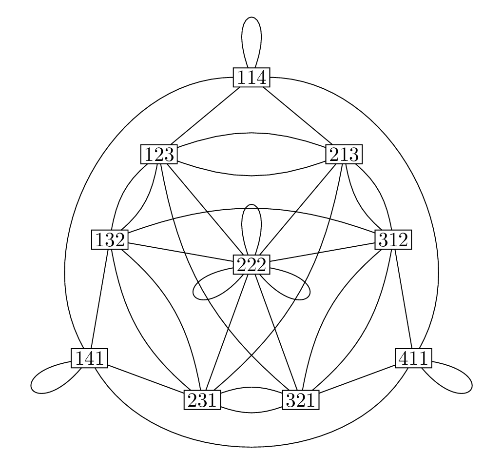
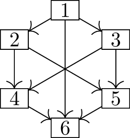
A multigraph representation of the \(6\)-pebble game
Figure 7.1 shows a graph of the
possible states of the \(6\)-pebble
game (with vertex \(xyz\) representing
a state with \(x\), \(y\), and \(z\) pebbles in the three piles); edges in
the graph represent valid moves. Well… it doesn’t quite show a graph of
the game: it has some edges that a graph cannot have. These edges
represent moves that do not change the state, as well as situations
where two different moves accomplish the same result.
Why would we draw a loop from vertex \(114\) back to itself?
Swapping the first two piles in state
\(114\) just takes us back to state
\(114\), since the two piles have the
same number of pebbles.
Why are there two edges between vertices
\(123\) and \(213\)?
The game has two ways to turn \(123\) into \(213\) (or the reverse): we can move a
pebble from the \(2\)-pebble pile to
the \(1\)-pebble pile, or we can swap
the \(1\)-pebble pile with the \(2\)-pebble pile.
Okay, so what’s going on at vertex \(222\)?
The six “reasonable” edges out of vertex
\(222\), going to vertices \(123\), \(132\), \(213\), \(231\), \(312\), and \(321\), all represent moving a pebble from
one pile to another. There are also three moves that accomplish nothing:
we can pick any two piles and swap them.
We cannot have these edges in a graph, so we define a multigraph to
be a more general kind of structure that allows these edges to exist.
The formal definition needs to be a bit more complicated, though.
Definition 7.1. A multigraph\(G\) is a triple consisting of an
arbitrary set of vertices\(V(G)\), an arbitrary set of
edges\(E(G)\), and a
symmetric incidence relation between them: we say that
vertex \(x\) is
incident to edge \(e\), or \(e\) is incident to \(x\), if they are related by the incidence
relation.
In a multigraph, two vertices are called
adjacent if there is an edge incident to both.
Previously, we defined edges as pairs of vertices. This is no longer
possible, because two edges can have the same pair of endpoints; to
distinguish them, there must be something more to their identity. In
diagrams (such as in Figure 7.1) we often don’t mark the
difference between such edges, but to deal with them formally, we would
need to give them individual labels.
We have special names for the two situations that can exist in a
multigraph, but not in a simple graph:
Definition 7.2. An edge in a multigraph which
has only one endpoint is called a loop. Two edges are
called parallel if they have the same set of
endpoints.
For example, in Figure 7.1, there is a loop incident
to vertex \(114\), two parallel edges
joining vertices \(123\) and \(213\), and three parallel loops incident to
vertex \(222\).
There are relationships between graphs and multigraphs in both
directions:
Definition 7.3. A simple graph
is a graph. The simplification of a multigraph \(G\) is the simple graph with the same
vertex set, and an edge \(\{x,y\}\)
(for \(x, y\in V(G)\) with \(x \ne y\)) whenever \(G\) has at least one edge incident to both
\(x\) and \(y\). Effectively, this removes all loops,
and replaces parallel edges with a single edge.
When a multigraph has no loops or parallel edges, we will treat
it as the same object as its simplification; even though on a low level
they are defined differently, reasoning about them in practice yields
identical outcomes.
Many notions that we’ve introduced for graphs still make sense for
multigraphs, with some modifications. There are two relatively large
changes that are worth spending some time discussing: one related to
walks, paths, and cycles, and another related to vertex degrees.
A walk in a multigraph is no longer just a sequence of vertices: it
matters how we get from one vertex to another. For example, in the \(6\)-pebble game, we consider a multigraph
model if it matters which kind of move we used at each step. (If this
distinction does not matter, then we do not need the added complexity of
multigraphs.) Thus:
Definition 7.4. An \(x-y\) walk of length \(l\) in a multigraph \(G\) is a sequence \[(x_0, e_1, x_1, e_2, x_2, \dots, x_{l-1}, e_l,
x_l)\] that alternates between vertices and edges of \(G\), satisfying the following: \(x = x_0\), \(y =
x_l\), and for each \(i=1, \dots,
l\), the endpoints of edge \(e_i\) are \(x_{i-1}\) and \(x_i\).
For example, suppose that we start in state \(114\) of the pebble game, and we make three
moves: we swap the first two piles, then move one pebble from the last
pile to the first, then swap the first two piles again. To represent
this as a walk, we’ll in the \(6\)-pebble multigraph, we will first need
to invent notation for the different types of edges. Let’s say that
\(s_{ij}\{x,y\}\) denotes a move
between states \(x\) and \(y\) by swapping piles \(i\) and \(j\), and \(m_{ij}\{x,y\}\), denotes a move between
states \(x\) and \(y\) by moving a pebble between piles \(i\) and \(j\). (Keep in mind that edges don’t have a
distinguished start and end, so \(s_{ij}\{x,y\}\) is the same edge as \(s_{ij}\{y,x\}\).) Then our walk would be
represented by the sequence \[(114,\;
s_{12}\{114,114\},\;
114,\;
m_{31}\{114,213\},\;
213,\;
s_{12}\{213,123\},\;
123).\] This is very cumbersome, so usually we don’t pull out the
full notation unless we need it. Even if we’re not looking this closely,
though, the definition still matters. For example, when listing the
different walks between two vertices, it is important to know when two
walks are considered to be different: they are different if the two
sequences are different.
Paths and cycles have the same definition, but with new implications.
Previously, we were not able to define cycle graphs \(C_1\) or \(C_2\); this is possible in the world of
multigraphs. The multigraph \(C_1\) is
a single vertex with a loop; the multigraph \(C_2\) has two vertices and two edges
between them.
In all cases, to pick out a path and cycle in a multigraph, we need
to specify not only the vertices and the order in which they occur, but
also the specific edges we use between those vertices. The upshot is
that paths and cycles can still be represented by walks (closed walks,
in the case of a cycle), but they must be the multigraph walks defined
in Definition 7.4.
If there’s any bright side to this, it is that it’s easier to tell
when a closed walk represents a cycle. This is true of a closed walk
\[(x_0, e_1, x_1, e_2, x_2, \dots, x_{l-1},
e_l, x_0)\] as long as \(e_1, e_2
\dots, e_l\) are distinct, vertices \(x_0, x_1, \dots, x_{l-1}\) are distinct,
and \(l\ge 1\).
Degrees in multigraphs
We would like to generalize the definition of vertex degrees to apply
to multigraphs, while giving the same answer as our old definition for
simple graphs when there happen to be no loops or parallel edges. It is
not obvious how to do so in a natural way, so let’s stop and think for a
moment about it.
Definitions are not set in stone: as mathematicians, we can choose
how to make them. However, we should try to make interesting and useful
definitions. Pay attention to the reasoning here if you want to
understand why definitions are the way they are!
To begin with, for simple graphs, we can count the degree of a vertex
\(x\) in two equivalent ways: by
counting the edges incident to \(x\),
or by counting the vertices adjacent to \(x\). In a multigraph, these two methods can
give different answers: for example, in Figure 7.1, vertex \(123\) is incident to \(7\) edges, but only has \(5\) neighbors!
We must immediately reject the second method of counting, because it
completely ignores the multigraph structure: why bother having two edges
between \(123\) and \(132\) if it’s not going to affect the
degree of either vertex? In other words, counting vertices adjacent to
\(x\) yields the degree in the
simplification of the multigraph.
The first method of counting is not bad, and could have ended up the
definition. However, it also has a problem.
By this rule, the degree sequence of the \(6\)-pebble graph would be \(9, 7, 7, 7, 7, 7, 7, 5, 5, 5\). By the
handshake lemma (Lemma 4.1), which we proved
in Chapter 4 for simple graphs, the sum of
degrees in a graph is twice the number of edges; applying that here, we
would conclude that the graph has \(\frac{9 +
6 \cdot 7 + 3 \cdot 5}{2} = 33\) edges. But this is incorrect: if
you count the edges in Figure 7.1
one by one, you will get \(36\).
Where does the discrepancy between \(33\) and \(36\) come from?
It comes from loops: when we naively apply
the handshake lemma, the \(6\) loops in
the graph only get counted as \(3\).
Looking at the proof of the handshake
lemma, why does this happen?
In the proof, we assumed that adding an
edge to a graph increases the degree sum by \(2\). However, if the degree of a vertex
were defined to be the number of incident edges, then a loop would only
increase the degree of a single vertex by \(1\).
The handshake lemma is so valuable that we are willing to add a
special case to our definition, just for this purpose. To rescue the
lemma, we need the degree sum to increase by \(2\) when a loop is added to a graph. It
wouldn’t make any sense for a loop incident to a vertex \(x\) to increase the degree of any vertex
other than \(x\); thus, it must
contribute \(2\) to the degree of \(x\). This tells us what the definition of
vertex degree must be:
Definition 7.5. The degree of a
vertex \(x\) in a multigraph \(G\) is the number of edges incident to
\(x\), counting every loop incident to
\(x\) twice.
By this definition, the degree sequence of the \(6\)-pebble graph is \(12, 7, 7, 7, 7, 7, 7, 6, 6, 6\).
You might ask: is there a graphic sequence problem for multigraphs?
There is, but the answer to it is much less exciting than it is for
graphs. Practice problem 3 at the end of
this chapter gives the condition, and asks you to discover the proof
yourself.
Finally, the definition of a graph isomorphism changes when it is
applied to multigraphs. There are two equivalent ways to make that
change:
We could say that an isomorphism between multigraphs \(G\) and \(H\) is still a bijection \(\varphi\colon V(G) \to V(H)\), but with a
slightly different condition on \(\varphi\). Rather than simply preserving
adjacency, it should be the case that for any vertices \(x\) and \(y\) in \(G\) (possibly equal) the number of edges
between \(x\) and \(y\) should be the same as the number of
edges between \(\varphi(x)\) and \(\varphi(y)\).
We could also say that an isomorphism between multigraphs \(G\) and \(H\) is a pair of bijections: a bijection
\(\varphi\colon V(G) \to V(H)\), and a
second bijection \(\varphi' \colon E(G)
\to E(H)\). The condition relating these should now be that for a
vertex \(x \in V(G)\) and an edge \(e \in E(G)\), \(x\) is incident to \(e\) if and only if \(\varphi(x)\) is incident to \(\varphi'(e)\): the bijections \(\varphi\) and \(\varphi'\) preserve the incidence
relation.
These two options are equivalent, and therefore equally good, but the
second is more in the spirit of our definition of a multigraph. The
intuition you should have is that a discrete structure (like a graph or
a multigraph) consists of two parts: some objects, and some
relationships between them. In the case of a multigraph, the objects are
the vertices and edges, and the relationships between them are given by
the incidence relation. An isomorphism between two discrete structures
should be a bijection between the objects that preserves the
relationships. This idea will guide you to the correct definition of an
isomorphism both in graph theory and outside it.
Directed graphs
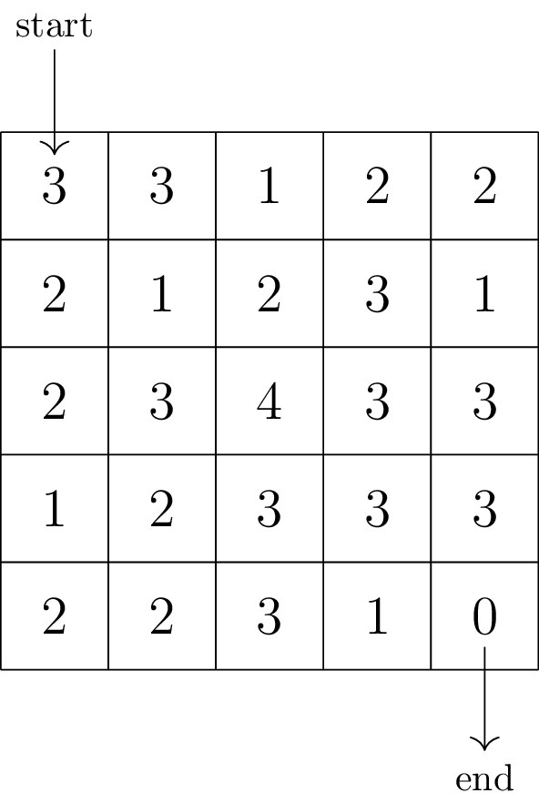
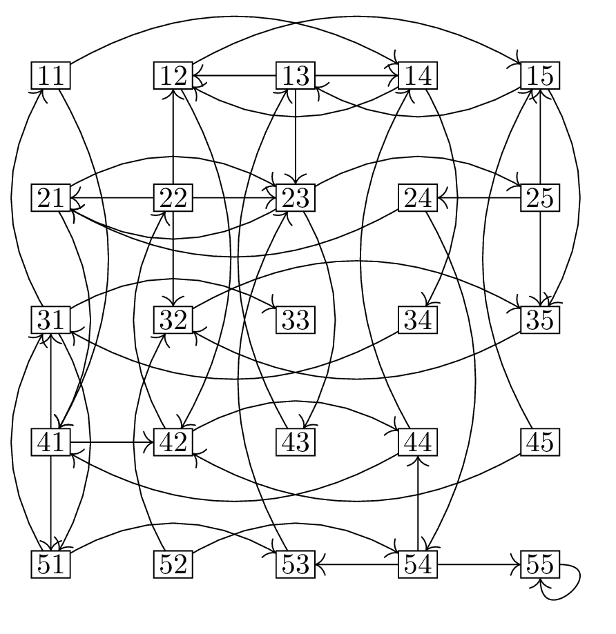
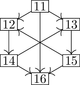
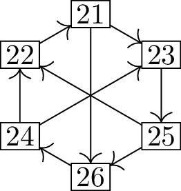
A numerical mazeA digraph representation of the maze
Solving a maze using directed graphs
Figure 7.2(a) shows an unusual kind of
maze: a numerical maze. Like a normal maze, it has a start (the top left
cell) and an end (the bottom right cell). Instead of paths and walls,
however, you solve the maze by using the numbers: if you’re in a cell
with the number \(k\), then you can
jump to another cell that’s \(k\) steps
away either horizontally or vertically.
We might try to represent an ordinary maze by a graph, so that a path
in the graph from the start vertex to the end vertex will give us a
solution to the maze. In the numerical maze, we encounter an unexpected
difficulty: the jumps we make in the maze are often one-way. From the
top left corner, which has a \(3\) in
it, we can jump to a cell three steps to the left or to a cell three
steps down. However, neither of these numbers contains a \(3\), so neither of them will let us return
to where we just were! As a result, a graph is unsuitable as a model for
this maze: adjacency between the cells is an asymmetric
relationship.
The structure we use in such cases is called directed graph, or
digraph for short. In a diagram, we draw a directed graph by making each
edge an arrow, rather than a line, as in Figure 7.2(b). An arrow from vertex \(x\) to vertex \(y\) represents, informally, an adjacency
that exists only when going from \(x\)
to \(y\), not when going from \(y\) to \(x\). The formal definition is:
Definition 7.6. A directed
graph or digraph\(D\) is a pair consisting of an arbitrary
set of vertices \(V(D)\) and a set of
arcs or directed edges\(E(D)\). Each arc is an ordered pair \((x,y)\) where \(x,y \in V(D)\).
We say that arc \((x,y)\)starts at \(x\) and
ends at \(y\); it is
an arc from \(x\) to \(y\), or out of \(x\) and into \(y\).
In principle, we could combine this definition with the definition of
a multigraph in the previous section, obtaining the concept of a
directed multigraph. I will not do so in this book; juggling all these
definitions is complicated enough as it is! However, even without that
added flexibility, we allow the arcs \((x,y)\) and \((y,x)\) to coexist in a digraph: after all,
these are not the same arc. For example, in Figure 7.2(b), arcs \((21,23)\) and \((23,21)\) both exist: we can jump in either
direction between this pair of cells, because they are \(2\) steps apart, and both contain a \(2\). The pair \((x,x)\) is also a valid ordered pair, so it
can also be an arc in a directed graph: it represents a loop from \(x\) to \(x\).
It is sometimes convenient to forget about the directions of the
arcs, and go back to an undirected object.
Definition 7.7. The underlying
graph of a digraph \(D\) is
the multigraph \(G\) with vertex set
\(V(G) = V(D)\) and an edge incident to
\(x\) and \(y\) for each arc \((x,y) \in E(D)\). The digraph \(D\) is called an orientation of \(G\).
In directed graphs, the notion of vertex degrees becomes even more
muddled than it was for multigraphs. Properly speaking, we should not
describe the degree of a vertex by a single number. Instead, we count
the number of arcs into a vertex and the number of arcs out of a vertex
separately.
Definition 7.8. The indegree of
a vertex \(x\) in a digraph \(D\), denoted \(\deg^{-}_D(x)\), is the number of arcs into
\(x\).
The outdegree of a vertex \(x\) in a digraph \(D\), denoted \(\deg^{+}_D(x)\), is the number of arcs out
of \(x\).
As with the ordinary notion of degree, we drop the subscript and
write \(\deg^-(x)\) and \(\deg^+(x)\) if it is clear which digraph
containing vertex \(x\) we mean.
An even more powerful version of the handshake lemma holds for
indegrees and outdegrees in directed graphs. Before reading ahead to see
how to prove it, see if you can figure out a proof of Lemma 7.1 yourself, by
imitating the proof of Lemma 4.1 in Chapter 4.
Lemma 7.1. In any digraph \(D\), the vertex indegrees add up to the
number of arcs, as do the vertex outdegrees: \[\sum_{v \in V(D)} \deg^-_D(v) = |E(D)| = \sum_{v
\in V(D)} \deg^+_D(v).\]
Proof. We will prove that for any directed graph with \(m\) edges, the identity in the lemma holds,
and we will do it by induction on \(m\).
The base case is \(m=0\). The lemma
holds in this case because the sum of indegrees, the number of arcs, and
the sum of outdegrees are all equal to \(0\): there are no arcs, so no vertex has a
nonzero indegree or outdegree.
Assume that the lemma holds for all directed graphs with \(m-1\) arcs. Let \(D\) be a directed graph with \(m\) arcs, and let \((x,y)\) be any arc of \(D\). We can apply the induction hypothesis
to \(D - (x,y)\), a digraph with \(m-1\) arcs.
What is the relationship between the indegrees and outdegrees in
\(D\) and in \(D-(x,y)\)? There are three cases:
In \(D\), the outdegree of \(x\) is \(1\) higher than in \(D - (x,y)\), because arc \((x,y)\) contributes \(1\) to that outdegree.
In \(D\), the indegree of \(y\) is \(1\) higher than in \(D - (x,y)\), because arc \((x,y)\) contributes \(1\) to that indegree.
\(\deg^+_{D - (x,y)}(v) =
\deg^+_D(v)\) and \(\deg^-_{D-(x,y)}(v)
= \deg^-_D(v)\) in all other cases.
Adding up all the changes, we see that \[\sum_{v \in V(D)} \deg^-_D(v) = 1 + \sum_{v \in
V(D)} \deg^-{D-(x,y)}(v)\] and \[\sum_{v \in V(D)} \deg^+_D(v) = 1 + \sum_{v \in
V(D)} \deg^+{D-(x,y)}(v).\] By the induction hypothesis, both of
the right-hand sides are equal to \(1 + (m-1)
= m\), proving the lemma for \(D\): an arbitrary \(m\)-arc directed graph. Then, by induction,
the lemma holds for directed graphs with any number of arcs. ◻
Less commonly, in addition to the indegree and outdegree of a vertex,
we define the net degree of \(x\) to be
\(\deg^{\pm}_D(x) = \deg^+(x) -
\deg^-(x)\) and the total degree of \(x\) to be \(\deg_D(x) = \deg^+(x) + \deg^-(x)\).
How can we interpret the net degree and
the total degree of \(x\)?
The net degree measures how many more arcs
at \(x\) go out, compared to in; it
tells us whether \(x\) is a “net
exporter” or “net importer” of arcs. The total degree is the degree of
\(x\) in the underlying graph.
What do the net degrees add up to in a
directed graph?
We can write the sum of net degrees as
\[\sum_{v \in V(D)} \deg_D^{\pm}(v) = \sum_{v
\in V(D)} \deg^+(v) - \sum_{v \in V(D)} \deg^-{(v)},\] which
simplifies to \(0\) by Lemma 7.1.
What do the total degrees add up to?
For a similar reason, they add up to \(2|E(D)|\). This also follows from the
handshake lemma applied to the underlying graph of \(D\).
In directed graphs, the notion of isolated vertices (with indegree
and outdegree \(0\)) still makes sense,
but it is sometimes useful to consider the indegree and outdegree
separately. We call a vertex \(x\) in a
digraph a source if \(\deg^-(x) =
0\), and a sink of \(\deg^+(x)
= 0\).
Does the graph in Figure 7.2(b) contain any sources?
Yes: vertices \(45\) and \(52\) are sources. (You might be tempted to
call \(11\) a source because it’s a
starting point, but it’s not: it’s possible to return to vertex \(11\) after leaving it.)
Does it contain any sinks?
Yes: vertex \(33\) is a sink, because the number in the
center of the grid is \(4\), and there
are no cells to hop to that are \(4\)
spaces away in any direction. Sinks in such a graph represent “dead
ends” in the maze which cannot be left.
Directed walks, paths, and
cycles
Moving on, the other big change with directed graphs—and, often, the
reason we study directed graphs to begin with—is the behavior of walks,
paths, and cycles. The definition of a walk in a digraph superficially
does not seem very different from the definition we saw in Chapter 3 for undirected graphs:
Definition 7.9. An \(x-y\) walk of length \(l\) in a digraph \(D\) is a sequence \[(x_0, x_1, x_2, \dots, x_l)\] of vertices
of \(D\) where \(x = x_0\), \(y =
x_l\), and for each \(i=1, \dots,
l\), \((x_{i-1}, x_i)\) is an
arc of \(D\).
The difference is that this definition requires all the arcs \((x_{i-1}, x_i)\) to point in the same
direction along the directed walk, and this small difference is a
dramatic change. While an \(x-y\) walk
in an undirected graph is essentially the same as an \(x-y\) walk except for which way you go, a
directed graph might have an \(x-y\)
walk but no \(y-x\) walk.
By analogy with \(P_n\) and \(C_n\), there are two families of directed
graphs: the directed path graph\(\overrightarrow{P_n}\) has vertex set \(\{1,2,\dots,n\}\) with an arc \((i,i+1)\) for \(i=1,2,\dots,n-1\), and the directed
cycle graph\(\overrightarrow{C_n}\) is obtained from
\(\overrightarrow{P_n}\) by adding the
arc \((n,1)\). Both of these are
defined for all \(n\ge 1\).
When dealing with directed graphs, the terms path and
cycle refer to copies of the directed path graph and the
directed cycle graph, respectively; I may use the terms “directed path”,
“directed cycle”, or “directed walk” for emphasis. A directed path or
cycle is represented by a walk \((x_0, x_1,
x_2, \dots, x_l)\) if it has vertices \(\{x_0, x_1, \dots, x_l\}\) and arcs \(\{(x_0, x_1), \dots, (x_{l-1}, x_l)\}\). In
the case of a cycle, it follows that the walk representing it is closed,
with \(x_l = x_0\).
To finish this introduction to directed graphs, let’s put the new
ideas about directed graphs together into a theorem: the directed
version of Theorem 4.4 from
Chapter 4.
Theorem 7.2. Every directed graph \(D\) with no sinks contains a
cycle.
Proof. Let the walk \((x_0, x_1,
x_2, \dots, x_l)\) represent a path in \(D\) of the largest possible length. Because
\(D\) has no sinks, we know in
particular that \(\deg^+(x_l) > 0\),
so there must exist some arc \((x_l,
y)\) that starts at \(x_l\).
If \(y \notin \{x_0, x_1, x_2, \dots,
x_l\}\), then the walk \((x_0, x_1,
x_2, \dots, x_l, y)\) would represent a longer path, contrary to
our assumption. Therefore \(y = x_i\)
for some \(i\), and the closed walk
\((x_i, x_{i+1}, \dots, x_l, x_i)\)
represents the cycle we wanted. ◻
Does the same result hold for directed
graphs with no sources?
Yes: we can write a similar proof, but
look for a vertex \(y\) with an arc
into \(x_0\), rather than out of \(x_l\).
Does the converse hold? That is, if \(D\) has a cycle, is it true that it has no
sources or sinks?
No, and the digraph in Figure 7.2(b) is a counterexample. This
digraph has two sources and a sink, and yet it still has many cycles:
for example, the length-\(3\) cycle
represented by \((12, 15, 13,
12)\).
Practice problems
Consider the \(6\)-pebble
multigraph in Figure 7.1.
How many \(114-411\) walks of
length \(1\) does it have?
What about length \(2\)?
What about length \(3\)?
For practice, write out one of the length-\(3\) walks as a sequence of vertices and
edges, using the \(s_{ij}\{x,y\}\) and
\(m_{ij}\{x,y\}\) notation for
edges.
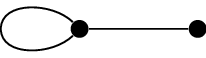
Consider the multigraph below. How many closed walks of length
\(10\) begin and end at the vertex on
the left?
Here is why we consider the graphic sequence problem for simple graphs,
and not for multigraphs.
Let \(d_1 \ge d_2 \ge \dots \ge
d_n\) be a sequence of nonnegative integers. Show that it is the
degree sequence of a multigraph if and only if \(d_1 + d_2 + \dots + d_n\) is even.
Let \(d_1 \ge d_2 \ge \dots \ge
d_n\) be a sequence of nonnegative integers. Show that it is the
degree sequence of a multigraph with no loops if and only if \(d_1 + d_2 + \dots + d_n\) is even and \(d_1 \le d_2 + d_3 + \dots + d_n\).
Let \(G\) be a simple graph with
\(n\) vertices and maximum degree \(r\). We assume that \(rn\) is even, so that an \(r\)-regular graph on \(n\) vertices exists. (But \(G\) might not be \(r\)-regular; some of its vertices can have
degree less than \(r\).)
Prove that there is an \(r\)-regular multigraph \(H\), with \(V(H)
= V(G)\), such that \(G\) is a
subgraph of \(H\). (In other words: we
can add edges to \(G\) to make it
regular.)
Give an example of a graph \(G\)
for which the graph \(H\) in part (a)
cannot possibly be a simple graph.
Solve the numerical maze in Figure 7.2(a).
What kind of graph-theoretic object represents your solution?
For an extra challenge, use breadth-first-search, as described in
Chapter 3, and find the shortest path
through the maze.
A game is played with two piles of stones. On a turn, a player
picks a pile which is not empty, and takes one or more stones from it.
The game ends once both piles are empty.
We can represent this game by a digraph whose vertices are the
states, with arcs representing the valid moves. Let \(D_{n,m}\) be the digraph we get when the
game is played with a pile of size \(n\) and a pile of size \(m\).
Draw a diagram of \(D_{3,2}\).
(It should have \(12\)
vertices.)
Which vertices of \(D_{n,m}\)
are sources? Which are sinks?
Are there any values of \(n\)
and \(m\) for which \(D_{n,m}\) contains a cycle?
The game RPS-7 [71],
invented by David C. Lovelace, is an extension of Rock-Paper-Scissors to
\(7\) gestures: Rock, Paper, Scissors,
Air, Fire, Sponge, and Water. The gestures have the following
relationships:
Rock pounds out Fire, crushes Scissors, and crushes
Sponge.
Fire melts Scissors, burns Paper, and burns Sponge.
Scissors swish through Air, cut Paper, and cut Sponge.
Sponge soaks paper, uses Air pockets, and absorbs Water.
Paper fans Air, covers Rock, and floats on Water.
Air blows out Fire, erodes Rock, and evaporates Water.
Water erodes Rock, puts out Fire, and rusts Scissors.
Let \({RPS}_7\) be the graph whose
vertices are the \(7\) gestures, with
an arc \((x,y)\) whenever gesture \(x\) beats gesture \(y\).
Find a cycle of length \(k\) in
\({RPS}_7\) for each \(k=3,4,5,6,7\).
For which \(n\) can an RPS-\(n\) game be constructed so that each object
beats the same number of other objects?
Write a reasonable definition of an isomorphism between two
directed graphs.
Here are three directed graphs with isomorphic underlying
graphs.
Prove that as directed graphs, none of these are isomorphic.
Footnotes
It’s a “game” because it has rules, but there is no
victory condition. Sorry.↩︎