Applications of bipartite matchings to other areas of math are
often all-or-nothing: either we find a perfect matching, or else we
have made no progress. Additionally, the graphs we face are not
arbitrary: they obey some mathematical laws defining their edges.
In such a scenario, Hall’s theorem is usually the way to proceed.
Hall’s condition is a necessary and sufficient condition for the
matching we want, and the abstract definition of our graph means it’s
often easy to verify. In this chapter, we will deduce Hall’s theorem
from Kőnig’s theorem and then—because this is not enough to make a
complete chapter—we will see some applications, ranging from
recreational mathematics to serious combinatorics.
Hall’s theorem is also often referred to as Hall’s marriage theorem,
and Hall’s condition is then called the marriage condition. I’m not
philosophically opposed to this (it can sometimes be handled poorly when
teaching, but it can also be handled well), but I don’t like the
terminology, so I’ve left it out of this chapter.
Hall’s theorem
Chapter 14 was devoted to proving Kőnig’s
theorem (Theorem 14.2), which is the result you
want to use for finding a maximum matching in a bipartite graph. In many
applications, that is absolutely the wrong question to ask, because only
a perfect matching counts as a solution; if no perfect matching exists,
we don’t care if the largest matching leaves \(2\) vertices or \(992\) vertices uncovered.
Of course, Kőnig’s theorem can also tell us when a perfect matching
exists, in terms of the number of vertices in a minimum vertex cover,
but this feels like the wrong way of thinking. In a graph \(G\) with bipartition \((A,B)\), where \(|A|=|B|=n\), we want to distinguish between
\(\beta(G) = n\) and \(\beta(G) \le n-1\) to determine whether a
perfect matching exists, and this doesn’t feel like a dramatic change.
What’s more, a vertex cover containing \(n-1\) vertices isn’t a very intuitive
explanation of why there is no perfect matching.
However, there are some situations in which we can tell a clear story
about why a perfect matching fails to exist.
What if the graph contains an isolated
vertex, \(x\)?
Then there is no perfect matching, because
there is no matching that covers \(x\).
What if vertices \(x\) and \(y\) have degree \(1\) and share the same neighbor \(z\)?
Then a matching can contain edge \(xz\) and cover \(x\), or contain edge \(yz\) and cover \(y\), but not both: so there is still no
perfect matching.
Generalizing these concepts, we can describe a minimum requirement
for a graph to have a perfect matching. First, we need a new
definition.
Definition 15.1. The
neighborhood\(N_G(S)\) of a set \(S \subseteq V(G)\) in a graph \(G\) is the set of all vertices of \(G\) adjacent to at least one vertex in
\(S\). If the graph \(G\) is clear from context, we simply write
\(N(S)\).
For example, a vertex \(x\) is
isolated if \(N(\{x\}) = \varnothing\).
Two leaf vertices \(x\) and \(y\) share their only neighbor \(z\) if \(N(\{x,y\}) = \{z\}\). What do these
situations have in common? A set of vertices has a neighborhood which is
too small: \(N(S)\) is smaller than
\(S\) itself.
Let \(S\)
be an arbitrary subset of \(A\). Can
there be a perfect matching if \(|N(S)| <
|S|\)?
No: a perfect matching must pair each
vertex of \(S\) with a different vertex
in \(N(S)\), which is impossible if
there are not \(|S|\) different
vertices in \(N(S)\) to use.
This explains why this condition is necessary for a perfect matching
to exist. Hall’s theorem (proved by Philip Hall in 1935 [47]) states that the condition
is also sufficient:
Theorem 15.1 (Hall’s theorem). A bipartite graph
\(G\) with the bipartition \((A,B)\) has a matching that covers all
vertices in \(A\) if and only if it
satisfies Hall’s condition: for all subsets \(S \subseteq A\), \(|N(S)| \ge |S|\).
In particular, when \(|A|=|B|\),
\(G\) has a perfect matching if and
only if it satisfies Hall’s condition.
What if \(|A|>|B|\)?
Then Hall’s condition will not be
satisfied if we take \(S=A\), because
\(N(A) \subseteq B\) and therefore
\(|N(A)| < |A|\).
What if \(|A|<|B|\)?
Then there is no perfect matching. In this
case, Hall’s theorem promises us a matching that covers every vertex in
\(A\), but leaves some vertices in
\(B\) uncovered.
Applying Hall’s theorem when \(|A|<|B|\) can still be very useful if
the vertices in \(A\) are different in
type from the vertices in \(B\). For
example, in the magic trick, we really want a matching that covers every
vertex \(\{a,b,c\}\) corresponding to a
set of \(3\) cards: then the matching
tells my assistant what to do when handed such a set. It would be fine
if the matching did not cover some ordered pairs \((a,b)\): that would mean that my assistant
will never hand me those two cards.
By proving Kőnig’s theorem, we have done all the hard work of proving
Hall’s theorem, and can now deduce it as a corollary. (It would also
have been possible to go the other way, and prove Kőnig’s theorem as a
corollary of Hall’s theorem.)
Proof of Theorem 15.1. We already know that Hall’s
condition is necessary for a matching to cover \(A\) to exist: if Hall’s condition is
violated for some subset \(S \subseteq
A\), then there is not even a matching that covers every vertex
in \(S\). It remains to prove that
Hall’s condition is sufficient. We will do this by assuming that there
is no matching that covers \(A\), and
finding a set \(S\) for which Hall’s
condition is violated.
Every edge in a matching has one endpoint in \(A\) and one endpoint in \(B\). So if there is no matching that covers
\(A\), then there is no matching with
\(|A|\) edges: \(\alpha'(G) < |A|\). By Kőnig’s
theorem, \(\beta(G) < |A|\): there
is a vertex cover \(U\) such that \(|U| < |A|\).
This set \(U\) is a small set of
vertices with a lot of neighbors, since every edge of \(G\) has at least one endpoint in \(U\). To find a set \(S\) for which Hall’s condition is violated,
we want the opposite: a large set of vertices with few neighbors. So we
define \(S\) to be \(A-U\): the set of all vertices in \(A\) that are not part of the vertex
cover.
For all vertices \(x \in S\), if
\(y\) is adjacent to \(x\), then \(U\) contains one endpoint of \(xy\), but \(U\) does not contain \(x\), so \(U\) must contain \(y\). Therefore all of \(N(S)\) is contained in \(U\). In addition to the vertices of \(N(S)\) (which are all on side \(B\)), \(U\) contains all of \(A-S\) (on side \(A\)); therefore \[|U| \ge |N(S)| + |A-S| = |N(S)| + |A| -
|S|.\] However, we also know \(|U| <
|A|\), so \(|N(S)| + |A| - |S| <
|A|\). This can be rearranged to get \(|N(S)| < |S|\), proving that \(S\) violates Hall’s condition. ◻
Suppose I give you a set \(S\) which violates Hall’s condition. Can
you use it to find a vertex cover with fewer than \(|A|\) vertices?
Yes: the set \((A - S) \cup N(S)\) is a vertex cover. For
every edge \(xy\), where \(x \in A\) and \(y\in B\), we have two cases: if \(x \in S\), then \(y\) is in the vertex cover, and if \(x \notin S\), then \(x\) is in the vertex cover.
Regular bipartite graphs
It is important to be clear about how Hall’s theorem is meant to be
used. It is not meant to be wielded like a hammer, going through the
subsets of \(A\) one by one and
searching for one that violates Hall’s condition. Such an algorithm
would take an exponentially long time! No: if you have a concrete graph
in front of you, and it has no short mathematical description, use the
augmenting path algorithm in Chapter 14 to
find a maximum matching and a minimum vertex cover. (There’s one
exception: if you can quickly spot a small set that violates Hall’s
condition, of course you should use that.)
Instead, we use Hall’s theorem when dealing with a graph or a family
of graphs in which the edges follow a regular mathematical pattern, and
we can prove that Hall’s condition is satisfied.
Our first example predates both Kőnig’s theorem and Hall’s theorem:
it originally appeared in 1894, in a thesis by Ernst Steinitz about
point-line configurations [94], though it was not stated in the
language of graph theory.
Theorem 15.2. For all \(r\ge 1\), if \(G\) is an \(r\)-regular bipartite graph, then it has a
perfect matching.
I admit that I am so fond of this theorem that I’ve put two versions
of it in a practice problem already, once in Chapter 8 and
once in Chapter 14. But we have not had the
opportunity to use Hall’s theorem to prove it, so let’s do that.
Proof of Theorem 15.2. Here’s a starting
observation that proves it’s permissible to at least hope for a perfect
matching. If \(G\) has a bipartition
\((A,B)\), then we can count the edges
of \(G\) in two ways. First, we could
sum the degrees of all vertices in \(A\) and get \(r|A|\): this counts every edge once,
because every edge has an endpoint in \(A\). We could also sum the degrees of all
vertices in \(B\) and get \(r|B|\). The two methods must give the same
answer, so \(r|A|=r|B|\), and \(|A|=|B|\).
To prove that a perfect matching exists, we show that Hall’s
condition holds for an arbitrary subset \(S
\subseteq A\). As in the previous paragraph, there are \(r|S|\) edges with an endpoint in \(S\). Similarly, there are \(r|N(S)|\) edges with an endpoint in \(N(S)\). By definition, every edge with an
endpoint in \(S\) has the other
endpoint in \(N(S)\); in other words,
the \(r|N(S)|\) edges with an endpoint
in \(|N(S)|\) include among them all
\(r|S|\) edges with an endpoint in
\(S\). This gives the inequality \(r|N(S)| \ge r|S|\), or \(|N(S)| \ge |S|\). ◻
Theorem 15.2 is one of the few results
in matching theory that is useful for multigraphs, not just simple
graphs. You would not expect this to happen! After all, loops and
parallel edges can never help us find a larger matching: a matching has
maximum degree \(1\), which means it is
always a simple graph. In fact, bipartite graphs cannot contain loops in
the first place, though they can have parallel edges: a loop can never
have one endpoint in \(A\) and the
other in \(B\).
So why would it matter that Theorem 15.2 is true for
multigraphs?
It is possible that a bipartite multigraph
is only \(r\)-regular due to the
presence of parallel edges, and if we eliminate those, then checking
Hall’s condition becomes much harder.
I should emphasize that when we go from an \(r\)-regular multigraph to a simple graph,
Hall’s condition will still be true: it will just no longer follow
automatically from Theorem 15.2.
To confirm for ourselves that Theorem 15.2
still does work for multigraphs, we could go through all our proofs and
verify that nothing changes in the presence of parallel edges. (We would
need to go through many proofs because of the dependencies between
them.) However, there is a shortcut.
Let \(G\) be a bipartite \(r\)-regular multigraph, and let \(G'\) be the simplification of \(G\). We can quickly check that the
two-paragraph proof of Theorem 15.2
still works for multigraphs, and therefore \(G\) satisfies Hall’s condition. Therefore
\(G'\) also satisfies Hall’s
condition: adjacent vertices in \(G\)
are still adjacent in \(G'\), so
neighborhoods don’t change at all. Therefore \(G'\) has a perfect matching, which
corresponds to a perfect matching in \(G\).
It is possible to generalize the result of Theorem 15.2. Suppose that some
vertices in \(A\) can have degree more
than \(r\), and some vertices in \(B\) can have degree less than \(r\). Then \(r|S|\) is a lower bound on the number of
edges with an endpoint in \(S\), while
\(r|N(S)|\) is an upper bound on the
number of edges with an endpoint in \(N(S)\), but this only extends the
inequalities we have; we are still able to obtain \(r|N(S)| \ge r|S|\) and verify Hall’s
condition.
Does this give us a perfect matching?
No, because it’s now possible that \(|A| < |B|\).
However, we can still obtain the following corollary:
Corollary 15.3. For all \(r\), if \(G\) is a bipartite graph with bipartition
\((A,B)\) such that every vertex in
\(A\) has degree at least \(r\), while every vertex in \(B\) has degree at most \(r\), then \(G\) has a matching that covers \(A\).
Armed with Hall’s theorem and several of its variants, we are now
ready to tackle some problems outside graph theory.
A three-card magic trick
Here is a mathematical card trick I know. A version of it using the
ordinary \(52\)-card deck was invented
by Fitch Cheney [68], but I
will present a simplified version with a deck of \(8\) cards, numbered \(1\) through \(8\).
You choose \(3\) cards from the
deck, however you like, and give them to my assistant, while I look away
or even temporarily leave the room. The assistant then hands me two of
the cards, one at a time, and hands the third card back to you, for
reference.
I have not seen the third card you’re holding, at any point.
Nevertheless, I can now perform some quick mental arithmetic and name
the number on that card!
How is this possible? The answer doesn’t involve any hidden
communication: my assistant doesn’t try to communicate the third card
via eyebrow gestures and split-second timing. The answer involves only
mathematics. Before describing a particular implementation of this
trick, let’s understand how it is even possible to make the trick
work.
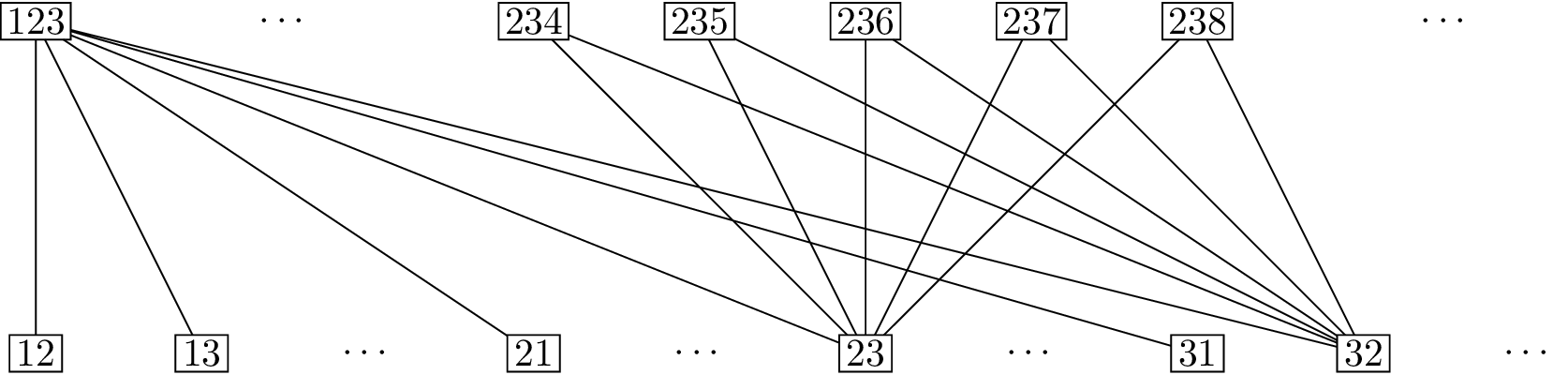
Consider the following bipartite graph. On one side of the
bipartition, the vertices are sets of three cards: \(\{1,2,3\}\) through \(\{6,7,8\}\). In the magic trick, you choose
three cards, which we can represent by a choice of one of these
vertices. On the other side, the vertices are ordered pairs of two
cards: \((1,2)\), \((1,3)\), and so on through \((8,7)\). In the magic trick, this
represents the information I get: the order in which the assistant hands
me the cards makes the pair an ordered pair.
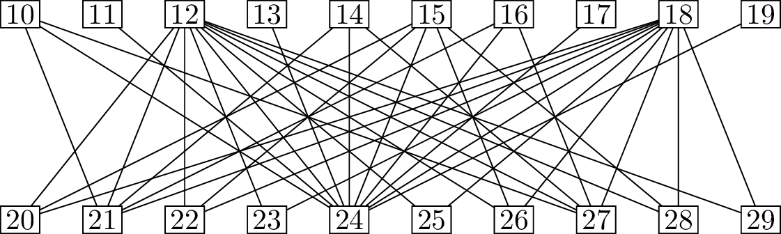
The bipartite graph for the three-card magic
trick
For the edges, join each set of three cards to the \(6\) ordered pairs that can be formed from
it: these represent the \(6\) choices
my assistant has, in deciding which two cards to give me and in which
order. The graph has \(112\) vertices,
so it is too big to draw in full, but Figure 15.1 shows
a portion of it: enough to see all the neighbors of vertices \(\{1,2,3\}\) on the first side and of \((2,3)\) and \((3,2)\) on the second side.
My assistant’s strategy, whatever it might be, picks a designated
neighbor of each vertex on the first side of the graph; for example, if
\((1,2)\) is the designated neighbor of
\(\{1,2,3\}\), then if you choose the
cards numbered \(1\), \(2\), and \(3\), my assistant will hand me card \(1\) and then card \(2\). Let \(M\) (for “magic”) be the spanning subgraph
containing only the edges between a vertex on the first side and its
designated neighbor; by construction, every vertex on the first side has
degree \(1\) in \(M\).
I presumably know \(M\) ahead of
time, so if I am handed card \(1\) and
then card \(2\), I should think about
the edges of \(M\) incident to vertex
\((1,2)\). If the edge between \(\{1,2,3\}\) and \((1,2)\) is the only such edge in \(M\), then I know that the third card must
have been \(3\). If, however, there are
multiple edges of \(M\) incident to
\((1,2)\), then I have many theories,
and cannot identify the third card. In other words, the magic trick only
works if every vertex on the second side has degree at most \(1\) in \(M\): if \(M\) is a matching!
Does such a matching exist? A first step is to check the number of
vertices. There are \(\binom 83 = \frac{8
\cdot 7 \cdot 6}{3!} = 56\) vertices on the first side: the
number of ways to choose a set of \(3\)
objects out of \(8\). There are \(8\cdot 7 = 56\) vertices on the second
side: the number of ways to choose a pair of \(2\) distinct objects out of \(8\). So it’s conceivable to have a matching
\(M\) that covers all \(56\) vertices on the first side, as long as
it also covers all \(56\) vertices on
the second side: it must be a perfect matching. We haven’t ruled out the
possibility that the magic trick works.
Why do we divide by \(3!\) in \(\frac{8
\cdot 7 \cdot 6}{3!}\), but don’t divide by anything in \(8\cdot 7\)?
In the first case, we’re counting sets,
which are unordered, so we divide by the \(3!\) ways to order the elements. In the
second case, we’re counting ordered pairs: my assistant hands me a first
card and a second card.
To see that the graph for the \(8\)-card magic trick has a perfect
matching, all we have to do is observe that it is \(6\)-regular and apply Theorem 15.2.
Why is the graph \(6\)-regular?
For every pair of cards I see, there are
\(6\) possibilities for the missing
third card. For every three cards my assistant sees, there are \(6\) possible actions: \(3\) ways to choose the first card to pass
me, multiplied by \(2\) ways to choose
the second card.
We can generalize to a \(k\)-card
magic trick: you choose \(k\) cards
from a (potentially very large) deck, my assistant hands me \(k-1\) of them in some order, and I must
guess the last card.
Proposition 15.4. The \(k\)-card magic trick can be performed if
the deck contains at most \(k! + k -
1\) cards.
Proof. Suppose the deck contains \(n\) cards; construct the bipartite graph
with bipartition \((A,B)\) where \(A\) is the set of all unordered \(k\)-card hands, \(B\) is the set of all ordered sequences of
\(k-1\) cards, and there is an edge
whenever a \(k\)-card hand contains all
cards in the \((k-1)\)-card
sequence.
Then every vertex in \(A\) has
degree \(k \cdot (k-1)! = k!\): when my
assistant takes a \(k\)-card hand and
hands me \(k-1\) cards in some order,
there are \(k\) ways to choose which
card I don’t get to see, and \((k-1)!\)
ways to sort the cards I do see. Every vertex in \(B\) has degree \(n-k+1\): when I am handed \(k-1\) cards, the number of \(k\)-card hands they could have come from is
equal to the number of possibilities for the \(k\)th card, which is \(n -(k-1)\) because that card can be any of
the cards except for the \(k-1\) I
see.
If we let \(r = k!\), then every
vertex in \(A\) has degree at least
(actually, exactly) \(r\). Provided
\(n-k+1 \le r\), every vertex in \(B\) has degree at most \(r\); this inequality is equivalent to \(n \le k! + k - 1\). When this happens, by
Corollary 15.3, the graph has a
matching \(M\) that covers all vertices
in \(A\).
At least in principle, if my assistant and I agree on a matching
\(M\), then we have a strategy for the
\(k\)-card trick. When handed \(k\) cards, my finds that \(k\)-card hand as a vertex in \(M\), and looks at the only neighbor of that
vertex to see which \(k-1\) cards to
give me, and in which order. When I am handed that sequence of \(k-1\) cards, I can do the reverse: find
that sequence as a vertex in \(M\), and
look at the only neighbor of that vertex to see which \(k\) cards were chosen. (If \(n < k! + k -1\), not all sequence of
\(k-1\) cards are covered by \(M\), but every sequence my assistant
actually hands is guaranteed to be covered!) This tells me, in
particular, which card is the hidden card. ◻
What’s the problem with implementing this
strategy?
For an arbitrary matching, too much
memorization is necessary! Essentially, my assistant and I have to
memorize what to do in every possible situation.
In 2002, Michael Kleber [61] not only proved Proposition 15.4, but also described a strategy
for the \(k\)-card trick that can be
implemented in practice, and I will finish our discussion of magic
tricks by describing it in the three-card case.
My assistant’s job is to add up the numbers on the three cards, and
find the remainder when the sum is divided by \(3\). The card my assistant hands back to
you is the smallest of the three cards if the remainder is \(0\), the middle card if the remainder is
\(1\), and the largest card if the
remainder is \(2\). My assistant hands
me the other two cards in increasing order if the missing card is one of
the three smallest cards I won’t see, and in decreasing order
otherwise.
What will my assistant do if you choose
the cards \(1, 3, 6\)?
\(1+3+6=10\), which leaves a remainder of
\(1\) when divided by \(3\), so my assistant will hand you the
middle card: \(3\). Of the cards I
won’t see, the three smallest ones are \(2, 3,
4\), of which \(3\) is one, so
my assistant hands me \(1\), then \(6\).
My job is to label the unseen cards, in order from largest to
smallest, as \({<}2\), \({<}1\), \({<}0\), \({>}2\), \({>}1\), and \({>}0\). I then guess the one where the
inequality sign (\(<\) or \(>\)) matches the relationship between
the first and second card I am given, and the number (\(0\), \(1\), or \(2\)) matches the remainder when the sum of
my two cards is divided by \(3\).
What will I do if I am handed the cards
\(1\) and \(6\) in that order?
Since \(1<6\) and \(1+6\) leaves a remainder of \(1\) when divided by \(3\), I want the card labeled \({<}1\): the second-smallest unseen card.
So I guess card \(3\).
Though this strategy is workable, and generalizes well, I wonder if
there’s a simpler procedure specifically for the three-card magic trick.
Maybe you will find one!
Generalized tic-tac-toe
The ordinary game of tic-tac-toe is played on a \(3 \times 3\) grid. Players take turns
placing their mark to claim an empty space in the grid: a for the first
player and a for the second player. A player wins by claiming all three
spaces in a horizontal, vertical, or diagonal line; if this does not
happen when the board is filled, then the game is a draw.
The ordinary game of tic-tac-toe is not very interesting once you’ve
learned how to play: every game between two skilled players ends in a
draw. However, there are many ways to generalize it. The game gomoku is
played on a \(15 \times 15\) board, and
the winning condition is to get \(5\)
consecutive pieces in a row. Mathematicians have also tried playing
tic-tac-toe in three (or more?) dimensions. A \(3 \times 3 \times 3\) game is not very
interesting, because the first player has an insurmountable advantage
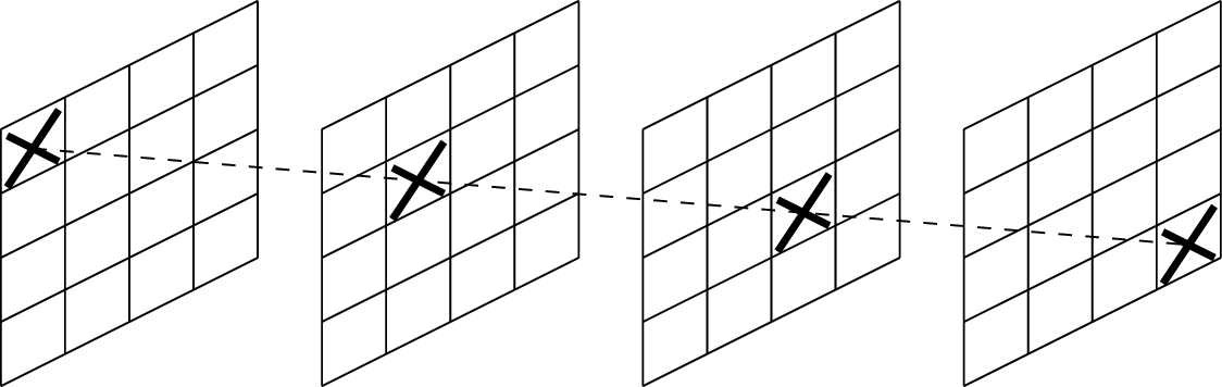
when claiming the center space, but \(4 \times
4 \times 4\) tic-tac-toe is worth playing. You just have to learn
to spot the winning lines (one example is shown in Figure 15.2).
A winning line in \(4 \times 4
\times 4\) tic-tac-toe
We will consider tic-tac-toe in even further abstraction: there is a
set of points \(\mathcal P\), which the
players take turns claiming, and a set of winning lines \(\mathcal L\). Each element of \(\mathcal L\) is a subset of \(\mathcal P\), and a player that claims all
the elements of a winning line wins.
Graph theory cannot solve all possible tic-tac-toe games at once, but
an application of Hall’s theorem can let us stop thinking about games
that are too boring: either player can easily guarantee a draw by a
strategy with very little interaction.
Proposition 15.5. In a generalized tic-tac-toe
game where every set of \(k\) winning
lines contain at least \(2k\) points in
total, either player can guarantee themselves at least a draw.
Proof. We will construct a somewhat unusual bipartite graph
to represent the game. On one side of the bipartition, we will have
\(\mathcal P\): the set of points. On
the other side of the bipartition, we will not put \(\mathcal L\), but rather two disjoint sets
called \(\mathcal L^+\) and \(\mathcal L^-\). For every winning line
\(\ell \in \mathcal L\), we put a
“positive vertex” \(\ell^+\) into \(\mathcal L^+\) and a “negative vertex”
\(\ell^-\) into \(\mathcal L^-\). Both \(\ell^+\) and \(\ell^-\) will be adjacent to the same set
of points in \(\mathcal P\): all the
points contained in \(\ell\).
Next, we set out to check Hall’s condition for a matching in this
graph to cover \(\mathcal L^+ \cup \mathcal
L^-\). Let \(S \subseteq \mathcal L^+
\cup \mathcal L^-\) be an arbitrary set. Then either \(|S \cap \mathcal L^+|\) or \(|S \cap \mathcal L^-|\) is at least \(\frac12|S|\): either at least half the
vertices in \(S\) are positive, or at
least half the vertices are negative. The two situations are symmetric,
so we assume \(|S \cap \mathcal L^+| \ge
\frac12|S|\).
If \(k = |S \cap \mathcal L^+|\),
then there are \(k\) winning lines
corresponding to vertices in \(S \cap \mathcal
L^+\), and by the condition we’ve assumed, there are at least
\(2k\) points on these lines. All these
points are in \(N(S \cap \mathcal
L^+)\), and therefore in particular they are in \(N(S)\). Therefore \(|N(S)| \ge 2k \ge |S|\), and Hall’s
condition holds.
Hall’s theorem gives us a matching in our unusually constructed
graph, but what do we do with this matching? Well, for every line \(\ell\), the matching gives us two points on
\(\ell\): the point matched to \(\ell^+\) and the point matched to \(\ell^-\). In other words, from every
winning line we’ve selected two points, such that each point has been
selected from at most one of the winning lines through it.
Using these selected points, you can obtain a draw whether you are
the first player or the second. Suppose your opponent has played on one
of the points selected from winning line \(\ell\). Then respond by claiming the other
point selected from \(\ell\), if you
have not claimed it already. In all other cases—if your opponent’s move
is not the point selected from any line, or if you’ve already claimed
the other point, or if it’s the first move of the game—play arbitrarily.
(A strategy of this type is called a pairing strategy in game
theory.)
What if your opponent plays on that point
with the goal of winning along some line other than \(\ell\)?
You don’t care, because that other line
has two selected points of its own.
If you use the pairing strategy, you will never lose, because your
opponent can never claim all the points on any line. To do so,
eventually your opponent would need to claim one of the selected points
from that line, but then you will just claim the other point. You will
probably not win, either, because the pairing strategy makes absolutely
no effort to do so; it’s possible that you will win accidentally.
However, you are guaranteed at least a draw. ◻
The condition of Proposition 15.5
seems hard to check, but for many tic-tac-toe games, it turns out \(k\) winning lines will contain far more
than \(2k\) in most cases, leaving only
a few cases to check. For example, consider a \(5\times 5\) board. A single line is
guaranteed to have \(5\) points; a
second line is guaranteed to add \(4\)
new ones; a third line is guaranteed to add \(3\) new ones, for a total of \(12\).
How can we argue rigorously that \(3\) lines contain at least \(12\) points?
They have \(5+5+5=15\) points if we double-count the
intersections, and \(3\) lines have at
most \(3\) intersection points.
Since \(12\) points is enough for up
to \(6\) lines, we can skip ahead to
considering a set of \(7\) lines. These
cover most of the board, and with a little bit more thinking, we can
conclude that the worst case is a set of all \(k=12\) lines, which cover all \(25\) points. Therefore Proposition 15.5 applies to tic-tac-toe on a
\(5\times 5\) board.
Incomparable sets
Our setting in this section will be the world of subsets of an \(n\)-element sets; we might as well assume
they are subsets of \(\{1,2,\dots,n\}\), because the exact
elements won’t matter.
Two subsets \(X\) and \(Y\) are called comparable if \(X \subseteq Y\) or \(Y \subseteq X\), and incomparable
otherwise. For example, the set \(\{2,3\}\) is comparable to (and a subset
of) the set \(\{2,3,4\}\); it is
incomparable to \(\{1,3,4\}\). You can
imagine that if the elements represent objects you want to own, then
\(\{2,3\}\) is clearly not as good as
\(\{2,3,4\}\), but it is not certain
which of \(\{2,3\}\) or \(\{1,3,4\}\) is better. For example, what if
elements \(1\), \(3\), and \(4\) are different kinds of cookies, while
element \(2\) is an expensive car?
Suppose we want to pick a family1 of sets in which no two
sets are comparable. An example is the family \(\big\{\{1,2,3\}, \{2,4\},
\{1,3,4\}\big\}\).
What is largest family of subsets of \(\{1,2,3,4\}\) in which no two are
comparable?
\(\big\{\{1,2\},
\{1,3\}, \{1,4\}, \{2,3\}, \{2,4\}, \{3,4\}\big\}\), the family
of all \(2\)-element subsets.
In general, if we take the family of all \(k\)-element subsets, for any \(k\), then any two subsets in the family
will be incomparable. The number of sets in this family is given by the
binomial coefficient \(\binom nk =
\frac{n!}{k! (n-k)!}\). This is maximized when \(k = n/2\): for example, when \(n=4\) we have \[\binom 40=1, \;
\binom 41=4, \;
\binom 42=6, \;
\binom 43=4, \;
\binom 44=1.\] So we want the family of all \((n/2)\)-element subsets. We will call this
the middle layer family.
What if \(n\) is odd?
When \(n\) is odd, there are two equally good
middle layers: the family of \(\frac{n-1}{2}\)-element subsets, and the
family of \(\frac{n+1}{2}\)-element
subsets. (For example, if \(n=5\), then
\(\binom 52 = \binom 53 = 10\).
By convention, let’s round \(n/2\)
down if \(n\) is odd. The notation for
rounding down is \(\lfloor
n/2\rfloor\), so the formula \(\binom{n}{\lfloor n/2\rfloor}\) tells us
the size of the middle layer family.
In 1928, Emanuel Sperner proved [93] that this is the best we can do, for any
\(n\). He did not use Hall’s theorem to
do this, but we will.
Theorem 15.6. If \(\mathcal F\) is a family of subsets of
\(\{1, 2, \dots, n\}\) such that no two
different sets \(X, Y \in \mathcal F\)
are comparable, then \(|\mathcal F| \le
\binom{n}{\lfloor n/2\rfloor}\).
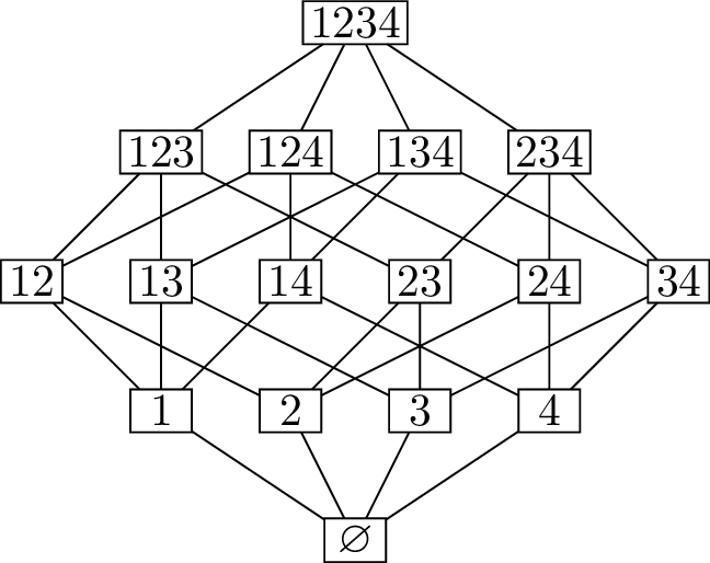
Proof. In Chapter 4, I
mentioned that the hypercube graph \(Q_n\) can be useful when reasoning about
set families, and that’s what we will do here. We defined the vertex set
of \(Q_n\) to be the set of \(n\)-bit strings: sequences \(b_1b_2\dots b_n\) where each \(b_i\) is either \(0\) or \(1\). To relate this to set families, a
vertex \(b_1 b_2 \dots b_n\) can be
identified with the subset of \(\{1, 2, \dots,
n\}\) containing an element \(i\) whenever \(b_i = 1\). The edges, which join \(n\)-bit strings that differ in only one
position, now tell us which two sets differ only by the presence or
absence of one element. For the rest of the proof, I will switch to
using set-related terminology. Figure 15.3(a) shows, for example,
\(Q_4\) with the vertices interpreted
as subsets (and \(\{x,y,z\}\) written
as \(xyz\) to simplify the
diagram).
We proved in Proposition 13.2 that
\(Q_n\) as a whole is bipartite, but a
perfect matching in \(Q_n\) will not
help us. Instead, we will write \(Q_n\)
as a union of bipartite graphs: \[Q_n =
G_{n,0} \cup G_{n,1} \cup \dots \cup G_{n,n-1}\] where \(G_{n,k}\) is the subgraph of \(Q_n\) induced by the sets of size \(k\) or \(k+1\). In other words:
\(G_{n,k}\) has the bipartition
\((A,B)\) where \(A\) is the set of \(k\)-element subsets of \(\{1,2,\dots,n\}\), and \(B\) is the set of \((k+1)\)-element subsets;
An edge \(xy\) with \(x\in A\) and \(y
\in B\) exists whenever we can add one more element to \(x\) to make \(y\). (It will be important later that when
this happens, \(x\) is a subset of
\(y\).)
In \(G_{n,k}\), every vertex \(x \in A\) has \(n-k\) neighbors in \(B\): there are \(n-k\) elements of \(\{1,2,\dots,n\}\) not already in \(x\) which we can add. Every vertex \(y \in B\) has \(k+1\) neighbors in \(A\): it has \(k+1\) elements which we can remove.
Provided \(n-k \ge k+1\), or \(k \le \frac{n-1}{2}\), Corollary 15.3 applies, giving us a
matching in \(G_{n,k}\) that covers
\(A\).
What kind of matching can we get if \(k \ge \frac{n-1}{2}\)?
In this case, Corollary 15.3 would apply if we
switched the roles of \(A\) and \(B\), so there is a matching that covers
\(B\).
In either case, call this matching \(M_k\). As a general rule, \(M_k\) covers the side of \(G_{n,k}\) with fewer elements, which is the
side further from the middle layer(s).
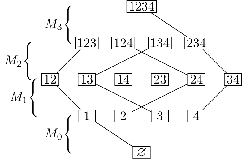
Now the magic happens! Consider the union \(M_0 \cup M_1 \cup M_2 \cup \dots \cup
M_{n-1}\), and call it \(H\).
Figure 15.3(b) shows one possible union \(H\) in the case \(n=4\).
Consider a vertex of \(Q_n\)
corresponding to a subset of size \(k\), for any \(k\). This vertex has degree \(1\) or \(2\) in \(H\): if \(k \le
\frac{n-1}{2}\), it is incident to one edge in \(M_k\) and maybe also one edge in \(M_{k-1}\), while if \(k \ge \frac{n-1}{2}\), then it is
guaranteed one edge in \(M_{k-1}\) and
possibly also an edge in \(M_k\). We
can follow these edges “up” the graph (increasing the number of
elements) and “down” the graph (decreasing the number of elements) until
we hit a dead end—a vertex of degree \(1\). So the connected component containing
the vertex we chose is a path, which means that every component of \(H\) is a path.
How many connected components are there? Well, from each vertex, we
can always follow edges of \(H\) to get
closer to the middle layer(s): those are the guaranteed edges. Therefore
each component of \(H\) contains one
vertex in the middle layer (or in each middle layer, for odd \(n\)). There are \(\binom{n}{\lfloor n/2\rfloor}\) vertices in
the middle layer, and therefore there are \(\binom{n}{\lfloor n/2\rfloor}\)
components.
So far, we have only looked at the structure of subsets of \(\{1,2,\dots,n\}\), but now we are ready to
consider the set family \(\mathcal F\)
that Theorem 15.6 is all about. You see, \(\mathcal F\) can never contain two sets in
the same connected component of \(H\).
If it did, then we could start at the set with fewer elements, and
follow it up the path to get to the one with more elements. At each
step, we’re adding an element, so the first set will be a subset of the
second—but we’ve assumed that \(\mathcal
F\) does not contain two such sets.
Therefore \(\mathcal F\) contains at
most one set from each connected component of \(H\); since there are \(\binom{n}{\lfloor n/2\rfloor}\) components,
we know that \(\mathcal F\) contains at
most \(\binom{n}{\lfloor n/2\rfloor}\)
elements. ◻
Practice problems
Is it possible to circle a letter in each of the words below so
that all \(9\) circled letters are
different? Either find a way to do it, or prove that it’s impossible
using Hall’s condition.
AREA
APART
ERRATA
GRAPH
PAPER
RETREAT
THEORY
TREE
YOGA
The multiples-of-six graph from Chapter 13
is shown again below:
Prove that it does not have a perfect matching, but this time, using
Hall’s theorem.
Let \(G\) be a bipartite graph
with \(n\) vertices on each side of the
bipartition whose minimum degree \(\delta(G)\) is greater than \(n/2\).
Prove that \(G\) has a perfect
matching.
Prove that when \(n > k! + k -
1\), it is impossible to perform the \(k\)-card magic trick with an \(n\)-card deck and guarantee that I guess
the \(k\)th card. (This is
not a problem about graph theory; it is a matter of counting.)
Find a pairing strategy for tic-tac-toe on a \(5\times 5\) board, where the goal is to win
by claiming all \(5\) spaces along a
horizontal, vertical, or diagonal line.
Let \(G\) be a bipartite graph,
with bipartition \((A,B)\), that has
the following properties:
Every vertex on side \(A\) has
degree \(3\) or \(5\);
Every vertex on side \(B\) has
degree \(2\) or \(4\);
There are no edges between vertices of degree \(3\) and vertices of degree \(4\).
Prove that \(G\) has a matching that
covers all vertices in \(A\).
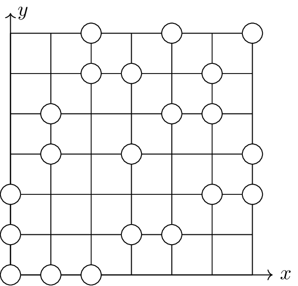
Suppose that we mark several points at integer coordinates in the
\(xy\)-plane in such a way that for
every marked point \((a,b)\), the lines
\(x=a\) and \(y=b\) each contain two other marked points.
This can be done by making a \(3\times
3\) grid, or in other, more complicated ways, such as in the
first diagram below.
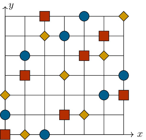
Prove that it is guaranteed to be possible to give the marked points
\(3\) different colors, as in the
second diagram above, so that no horizontal or vertical line passes
through two marked points of the same color.
(Putnam 2012) A round-robin tournament of \(2n\) teams lasted for \(2n-1\) days, as follows. On each day, every
team played one game against another team, with one team winning and one
team losing in each of the \(n\) games.
Over the course of the tournament, each team played every other team
exactly once. Can one necessarily choose one winning team from each day
without choosing any team more than once?
An \(n\times n\) Latin square is
an \(n\times n\) grid filled with the
integers \(1\) through \(n\) in such a way that every row and every
column contains each integer exactly once. For example, the first \(5 \times 5\) grid below is a Latin
square.
1
2
3
4
5
3
1
4
5
2
5
3
1
2
4
2
4
5
1
3
4
5
2
3
1
1
2
3
4
5
5
3
4
1
2
Suppose that, as in the second grid above, the first \(r\) rows in the \(n\times n\) grid are filled with integers
\(1\) through \(n\) in a way that does not cause any
contradictions: each of the \(r\) rows
use each integer exactly once, and no column contains any duplicates.
Prove that we can fill in the last \(n-r\) rows to get a Latin square.
Footnotes
A “family” of sets is just a set of sets, but we give it
a different word to make it easier to distinguish it from its
elements.↩︎