Trees are some of the most fundamental objects in graph theory.
There’s no single big theorem that makes them useful; instead, there are
many small facts. Trees appear when analyzing expression trees, or in
computer science applications; they are useful in more advanced graph
theory when analyzing connected graphs; they appear surprisingly often
in recreational math. In this chapter, I want to motivate trees by
introducing spanning trees, which is only one of many possible
motivations.
It is natural to follow up by considering the problem of finding
minimum-cost spanning trees, so I’ve included a section on that problem
at the end of this chapter; though it is not crucial for any content in
future chapters, it is nice to cover, if possible. (Students coming from
a discrete math class might have already seen Prim’s algorithm or
Kruskal’s algorithm; at the very least, the algorithm in this chapter is
different, providing some variety.)
In this chapter and the next, I’ve also tried to include several
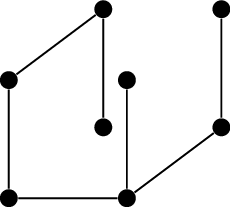
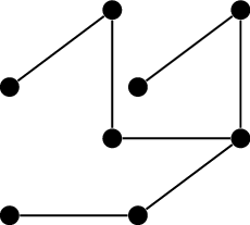
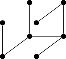
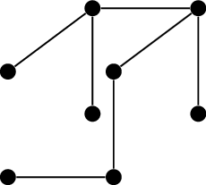
diagrams of different trees, in particular the six in Figure 9.2. Take a few moments to
just look at these and get a feeling for what trees are like, to
supplement the mathematical properties that we will be proving.
Spanning trees
What does it take to connect a graph?
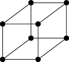
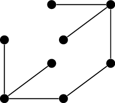
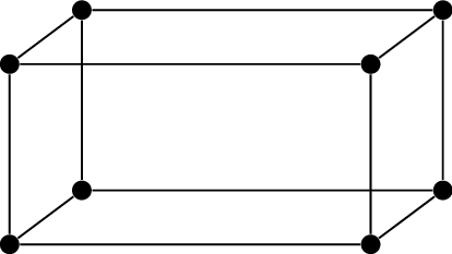
We have seen many examples of connected graphs. For example, the cube
graph, shown in Figure 9.1(a) as
a reminder, is connected.
The cube graphFrom 12 edges to 8From 8 edges to 7
What does it take to connect the vertices of a cube
graph?
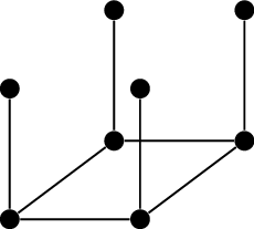
But not all the edges of the cube graph are necessary to have a
connected graph. For example, we can remove all edges between the four
vertices in the “top half” of the cube, and the result is still
connected, because those vertices can still get to each other through
the bottom half. The remaining graph, shown in Figure 9.1(b), has only \(8\) edges.
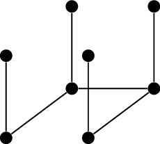
Even that is not the best we can do. Remove any one of the edges in
the bottom half, and the result is still connected: the bottom half of
the cube is a path. This results in a \(7\)-edge graph, shown in Figure 9.1(c).
Finally, in this graph, we can check that none of the \(7\) edges remaining could be removed. This
is certain to be true of whatever graph ends up our final stopping
point; if it weren’t, we would keep going. If we want to understand
connected graphs, we would do well to start with graphs that have this
property. They have a special name:
Definition 9.1. A tree\(T\) is a minimally connected graph: \(T\) is connected, but for every edge \(e \in E(T)\), the subgraph \(T-e\) is no longer connected.
(Why a “tree”? The term first appears in an 1857 paper of Arthur
Cayley [13], whom we
will meet again later on in our study of trees. Cayley’s trees were
diagrams used to represent various compositions of differential
operators: diagrams which started from a root and branched out to
smaller, similar diagrams, in just the way a tree grows.
Graph-theoretically, they had the same structure as what we call a tree
today.)
The graph in Figure 9.1(c) is a
tree. Moreover, it is a spanning subgraph of the cube graph we started
with in Figure 9.1(a): we did not delete any
vertices, only edges. In general, a spanning subgraph of a graph \(G\) which is a tree is a subgraph that
connects all vertices of \(G\) using as
few edges as possible; we call such an object a spanning
tree of \(G\).
It is natural to wonder whether some spanning trees are better or
worse than others; after all, we did not arrive at Figure 9.1(c) with any attempt to make good
decisions, but only did what is best in the moment. If you were to
experiment different approaches to the cube graph, you would find that
up to isomorphism, Figure 9.2 shows all possible
spanning trees of the cube graph.
Which of these trees has the fewest
edges?
All six of them have \(7\) edges: in this case, anything we do
must be equally good. In the next chapter, we will see that this is not
a coincidence.
Spanning trees of the cube graph
So why should we care about trees and spanning trees? For one, there
are many practical applications, because spanning trees are exactly what
you want if your goal is to connect a graph as cheaply as possible.
Imagine, for example, a transportation company whose network spans an
entire continent, but which has now fallen on hard times and needs to
cut back. It would like to offer as few routes as possible, but it does
not want to separate two parts of the country entirely. Under this
circumstance, the transportation company’s optimal solution will be a
spanning tree of its old route network.
Spanning trees will also be useful for us theoretically, and the
reason begins with the following theorem:
Theorem 9.1. A graph \(G\) is connected if and only if it has a
spanning tree.
Proof. Let \(G\) be any
connected graph. To find a spanning tree \(T\) of \(G\), we will delete edges of \(G\) one at a time until we get a tree.
This can be done essentially any way we like. Suppose we have ended
up at an intermediate graph \(H\) (some
spanning subgraph of \(G\)) and \(H\) has an edge \(e\) such that \(H-e\) is still connected. Then just delete
edge \(e\) and keep going. (If there
are many options for \(e\), pick any of
them.)
Eventually, we stop: we can’t keep deleting edges forever, because
\(G\) only has finitely many edges.
However, the only way this process can stop is when deleting any edge
would disconnect the remaining graph. That is exactly what it means to
be a tree: we have arrived at a spanning tree of \(G\).
In the other direction, suppose \(G\) has a spanning tree \(T\). Then any two vertices \(x,y\) of \(G\) are also vertices of \(T\), and \(T\) is connected, so there is an \(x-y\) walk in \(T\). That walk is also an \(x-y\) walk in \(G\), because \(T\) is a subgraph of \(G\). Therefore \(G\) is connected. ◻
Does anything about this theorem change
for multigraphs?
No, and in fact, if we start with a
multigraph, our very first step can be to delete loops and extra copies
of edges to make it a simple graph. These deletions can never disconnect
the graph.
The importance of Theorem 9.1 is
that it tells us about a single object (a spanning tree) which is enough
to show that a graph is connected. Without it, working directly from the
definition, we would have to consider different pairs of vertices \(x,y\) in the graph, and find an \(x-y\) walk between each of them.
This does not seem like a big deal at the moment, because to verify
that a subgraph \(T\) is a spanning
tree, we need to check that it is connected, which has all the same
difficulties. (Finding \(x-y\) walks in
\(T\) might be even harder than it was
in the original graph \(G\).) Later on,
as we learn more about trees, we will find ways to verify that \(T\) is a spanning tree which have nothing
to do with being connected. Then, Theorem 9.1
will come into its full power.
A final use of spanning trees is for proving general results about
connected graphs. If you have a problem about connected graphs that only
gets easier to solve when the graphs have more edges, then you can begin
by solving it in its hardest case: when the graph is a tree. If you do,
Theorem 9.1 will immediately give you a
general solution, by applying your specific solution to the spanning
tree of a general connected graph.
Bridges
Before we attain these promised powers, we need to learn much more
about trees. Fortunately, there are lots of things to learn.
To begin with, let’s take another look at the way we found a spanning
tree in the proof of Theorem 9.1. We
kept deleting edges if deleting them would not disconnect the graph,
until there were no more edges left that we could delete. We can give a
name to the type of edge that is left, as a prelude to studying such
edges more thoroughly:
Definition 9.2. A bridge\(e\) in a graph \(G\) is an edge of \(G\) such that \(G-e\) has more connected components than
\(G\). Most commonly, \(G\) is a connected graph, in which case
\(G\) is a bridge if and only if \(G-e\) is not connected.
As intuition for this name, you should imagine a long chain of
islands like the Florida Keys, connected to the mainland only by a
single bridge (the Overseas Highway, in the case of Florida). If
anything happened to the bridge, then the islands would only be
accessible by water.
If edge \(xy\) is a bridge of a connected graph \(G\), how many connected components does
\(G-xy\) have?
Two: each vertex \(z\) left in \(G-xy\) either has a walk to \(y\) or to \(x\). (If a \(z-y\) walk in \(G\) no longer exists in \(G-xy\), then that’s because it relied on
edge \(xy\), which means that it must
have at least reached \(x\).)
Similarly, if \(G\) is not
connected, and we delete an edge \(xy\), then the number of connected
components goes up by one: in \(G\),
there was a component \(H\) containing
\(xy\), which is replaced by the two
components of \(H-xy\).
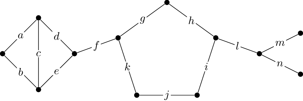
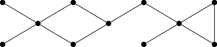
Which edges in this graph are bridges?In the graph shown in Figure 9.3, which edges are
bridges?
Edges \(f\), \(l\), \(m\), and \(n\).
Some graphs do not have any bridges at all. However, if we take a
connected graph and start deleting edges from it, this might cause some
of the remaining edges to become bridges. Eventually, if we keep
deleting edges that are not bridges, we will only have bridges left.
That’s what it means to be a tree! An equivalent way to phrase the
definition of a tree would be, “A tree is a connected graph in which all
edges are bridges.”
In Figure 9.3, what is the minimum
effort needed to show that \(g\) is not
a bridge?
It’s enough to show that it has a
substitute: any walk in the graph that uses edge \(g\) could instead use the edges \(h,i,j,k\). So it’s impossible to find two
vertices \(x\) and \(y\) such that all \(x-y\) walks rely on the existence of edge
\(g\).
In other words, edges \(g, h, i, j,
k\) make a cycle, and if something happens to one of these edges,
you can always “go the long way” around the cycle. In fact, this is
always the reason why an edge is not a bridge!
Lemma 9.2. An edge \(xy\) of a graph \(G\) is a bridge if and only if it is not on
any cycles.
Proof. We may assume that \(G\) is connected. If not, pass to the
connected component of \(G\) containing
\(x\) and \(y\); edge \(xy\) is still a bridge of that connected
component.
For one direction of the proof, we must formalize the idea of “going
the long way around”. Take a cycle in \(G\) containing edge \(xy\); we can represent it by a closed walk
\((x_0, x_1, \dots, x_{l-1}, x_0)\)
where \(x_0 = x\) and \(x_{l-1} = y\). Then \((x_0, x_1, \dots, x_{l-1})\) is an \(x-y\) walk that does not use edge \(xy\). We will use this walk to show that
\(G-xy\) is still connected, proving
that \(xy\) is not a bridge.
Let \(s,t\) be two vertices of \(G-xy\). Because \(G\) is connected, \(G\) has an \(s-t\) walk. In it, if we replace every
instance of \(\dots, x, y, \dots\) by
the \(x-y\) walk we found, and every
instance of \(\dots, y, x, \dots\) by
the reverse of this walk, we obtain an \(s-t\) walk which does not use edge \(xy\): it is still valid in \(G-xy\). Since \(s\) and \(t\) were arbitrary, \(G-xy\) is still connected.
For the other direction of the proof, suppose edge \(xy\) is not a bridge. Then \(G-xy\) is still connected, and in
particular, \(G-xy\) contains an \(x-y\) walk. By Theorem 3.1, \(G\) contains an \(x-y\) path \(P\). Adding edge \(xy\) to \(P\) produces a cycle (this is how the cycle
graph \(C_n\) is defined from the path
graph \(P_n\)), and that cycle contains
edge \(xy\). ◻
Properties of trees
What does Lemma 9.2 tell us about trees? In a tree
\(T\), every edge is a bridge, so no
edge is part of any cycles. Therefore a tree \(T\) has no cycles at all.
When considering multigraphs, can a tree
have loops or parallel edges?
No: a loop is a cycle of length \(1\), and a pair of parallel edges is a
cycle of length \(2\). So it is never
necessary to model a tree as a multigraph rather than a simple
graph.
Not all graphs without cycles are trees. However, the following is
true:
Proposition 9.3. A graph \(T\) is a tree if and only if it is
connected and has no cycles.
Proof. Both the condition in the proposition, and the
definition of a tree, say that \(T\) is
connected. So we must only show that a connected graph has no cycles if
and only if all its edges are bridges (the second part of the definition
of a tree).
If a graph has no cycles, then none of its edges lie on cycles: by
Lemma 9.2, they are all bridges. Conversely,
if all edges of a graph are bridges, then by Lemma 9.2, none of them lie on cycles—so no
cycles can exist at all, because a cycle needs to contain some edges.
This proves the equivalence we wanted. ◻
Proposition 9.3 is the first in a long line of
results that characterize trees, giving an if-and-only-if condition for
a graph to be a tree. Every such characterization could have been the
definition of trees we started with, though some are more suited to it
than others. Here is one more:
Proposition 9.4. A graph \(T\) is a tree if and only if it has no
cycles, but adding any edge would create a cycle.
Proof. Suppose \(T\) is a
tree; by Proposition 9.4, we already know it has no cycles.
Let \(e\) be any edge we could add to
\(T\); we want to show that \(T+e\) (the graph we get if we add edge
\(e\) to \(T\)) has a cycle. Well, \(e\) cannot be a bridge of \(T+e\): deleting it would only give us \(T\) again, and \(T\) is connected because it is a tree. So
by Lemma 9.2, \(e\) must lie on some cycle in \(T+e\), and in particular, adding \(e\) to \(T\) created a cycle.
For the reverse direction, suppose that \(T\) has no cycles, but adding any edge
would create a cycle. We want to prove that \(T\) is connected: then we can use
Proposition 9.3 and conclude that \(T\) is a tree. To this end, let \(x,y\) be two vertices of \(T\); we will be done if we find an \(x-y\) path in \(T\).
If \(xy\) is an edge of \(T\), then there is such a path: a path of
length \(1\). If not, then we know that
\(T+xy\) has a cycle. That cycle did
not exist in \(T\) (because \(T\) has no cycles at all), so it must use
the new edge \(xy\). As in the proof of
Lemma 9.2, when there is a cycle using edge
\(xy\), there is an \(x-y\) walk not using edge \(xy\) that “goes the long way around” the
cycle. This is an \(x-y\) walk that
still exists in \(T\), finishing our
proof that \(T\) is connected. ◻
We could rephrase Proposition 9.4 to say
that trees are exactly the graphs which are “maximally acyclic”: it has
no cycles, but no more edges can be added without losing that property.
In this way, it is a kind of opposite of our definition of trees as
“minimally connected”: connected with as few edges as possible, so that
no more edges can be removed without losing that property.
Minimum-cost spanning trees
At the beginning of a chapter, I asked you to imagine a
transportation company which wants to find the cheapest set of routes to
keep its network connected. Though I said that the transportation
company wants to find a spanning tree of its network, that’s not the
whole story. Not all spanning trees are equally cheap, because not all
of the routes in the transportation network are equally cheap to run or
to maintain. To keep track of this data, we need to consider more than
just a graph.
Definition 9.3. A weighted
graph is a graph \(G\)
together with a function \(c \colon E(G) \to
[0,\infty)\). For an edge \(e \in
E(G)\), the value \(c(e)\) is
called the cost or the weight of \(e\).
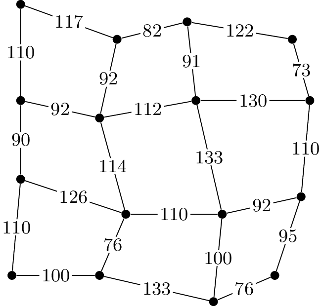
Figure 9.4(a) shows an example of a
weighted graph: what the transportation network’s route map might look
like. (To generate this simplified example, I placed the \(16\) vertices at slightly random points,
and computed the distance between the points to determine the cost of
the edges.)
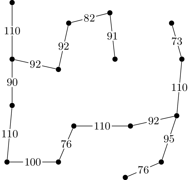
A weighted graphA minimum-cost spanning tree
Finding the minimum-cost spanning tree in a weighted
graph
When we measure the cost of a subgraph of a weighted graph, we
compute the total cost of its edges, adding up their individual costs. A
spanning tree \(T\) is a weighted graph
is called a minimum-cost spanning tree, or MCST for short, if
it has the minimum total cost. Figure 9.4(b)
shows a minimum-cost spanning tree of the weighted graph in Figure 9.4(a).
Should the MCST just use all the cheapest
edges in the graph?
No: some of the cheap edges might create a
cycle with even cheaper edges, making them redundant. On the other hand,
some very expensive edges might be necessary to connect the MCST.
There are many algorithms that can be used for finding the
minimum-cost spanning tree of a weighted graph. Famous ones include
Prim’s algorithm and Kruskal’s algorithm. In this chapter, I will show
you the reverse-delete algorithm (published by Joseph Kruskal
in the same paper [65]
as the algorithm that bears his name), because it bears the most
resemblance to our proof of Theorem 9.1.
In that proof, we repeatedly deleted edges, one at a time, until we
were left with a spanning tree; however, the proof did not specify which
edge to choose at each step. The only requirement is that we must never
delete a bridge.
If we were to modify that strategy to find a minimum-cost spanning
tree, which edges should we delete? The most natural guess is that of
all the non-bridges, we should pick the most expensive: the one with the
highest weight. This is a “greedy” strategy: it makes the best choice it
sees in the moment, with no regard to how this affects future
choices.
How could a greedy strategy fail—what
should we be concerned about?
It’s conceivable that if we delete a
cheaper edge and keep a more expensive one early on, then later in the
process this will let us delete several more expensive edges to make up
for it. The greedy strategy is not obviously correct: this will take
some proof.
Let us summarize the reverse-delete algorithm formally. This is a
slight change from the strategy we used to prove Theorem 9.1, because it only considers
each edge once—however, there will be no point in returning to a
previously-considered edge, because it will only be left alone if it is
a bridge.
Let \(e_1, e_2, \dots, e_m\) be
a list of the edges of \(G\) in
descending order of cost: from most expensive to cheapest. Also, let
\(G_0 = G\); we will construct a
sequence \(G_1, G_2, \dots, G_m\) of
graphs as we go.
Starting at \(i=1\), look at
edge \(e_i\) and ask: is \(e_i\) a bridge of \(G_{i-1}\)?
If \(e_i\) is a bridge, set \(G_i = G_{i-1}\); if \(e_i\) is not a bridge, set \(G_i = G_{i-1} - e_i\).
Repeat step 2 for \(i=2, 3, \dots,
m\), until all edges have been considered. Return \(G_m\) as the minimum-cost spanning
tree.
We will assume that there are no ties between the costs of the edges.
(One of the problems at the end of this chapter will ask you to
generalize this result to allow for ties.)
Theorem 9.5. Let \(G\) be a connected weighted graph in which
all edges have distinct costs. Then the output of the reverse-delete
algorithm for \(G\) will be a
minimum-cost spanning tree of \(G\).
Proof. The algorithm always produces a connected graph,
because it starts with a connected graph and never deletes a bridge.
Also, the only edges that are kept are bridges. Specifically, if edge
\(e_i\) survives to the final graph
\(G_m\), it must first survive to \(G_i\), which means it must have been a
bridge of \(G_{i-1}\). Therefore there
is no cycle in \(G_{i-1}\) containing
\(e_i\). To obtain \(G_m\) from \(G_{i-1}\), we only delete edges; therefore
\(G_m\) also cannot have a cycle
containing \(e_i\), making \(e_i\) a bridge of \(G_m\). Since this is true for every edge
\(e_i\), \(G_m\) must be a tree. Let’s give \(G_m\) another name: call it \(T\).
To prove that the algorithm is optimal, we need to compare \(T\) to an alternate spanning tree \(T'\), and somehow argue that \(T\) is better than \(T'\). Specifically, what we’ll do is
prove that if \(T' \ne T\), then
\(T'\) cannot be the MCST, because
we can make a small improvement to it. This will prove the theorem,
because it leaves \(T\) as the only
possible candidate for the MCST.
How can we do this? Well, first of all, if \(T \ne T'\), we can find an edge \(e\) which is present in \(T\), but not \(T'\). (If every edge of \(T\) were present in \(T'\), then either \(T'\) would be equal to \(T\), or \(T'\) would consist of \(T\) plus some additional edges. In the
latter case, \(T'\) would not be a
tree, because it would not be minimally connected.)
By Proposition 9.4, the graph \(T' + e\) has a cycle. Let \(C\) be that cycle, and let \(e'\) be the most expensive edge of
\(C\).
By looking at the reverse-delete algorithm, we can prove that \(e'\) cannot be part of \(T\), and in particular \(e' \ne e\). Here’s why: suppose that
\(e' = e_i\) in the list of edges
by cost. In the graph \(G_{i-1}\)
produced by the algorithm, \(e_i\) is
still present, and so are all the other edges of \(C\), because we have not gotten to any of
them yet. Therefore \(C\) is a cycle of
\(G_{i-1}\) containing \(e_i\), meaning (by Lemma 9.2) that \(e_i\) is not a bridge of \(G_{i-1}\). We conclude that \(e_i\) (that is, \(e'\)) is deleted and does not survive
to \(T = G_m\).
Therefore we can modify \(T'\)
as follows: add \(e\), but then delete
\(e'\). This produces a cheaper
connected graph!
Why is it cheaper?
Because \(e'\) is the most expensive edge of
\(C\), and \(e\) is some other edge of \(C\): we deleted a more expensive edge than
we added.
Why is it still connected?
Because we deleted an edge from a cycle of
\(T' + e\), which (by Lemma 9.2) was not a bridge.
Actually, it is true that \((T' + e) -
e'\) is a tree itself, but proving that is inconvenient at
the moment; it will be much easier once we can use Theorem 10.2 from the next chapter.
However, we do not need to know that it is a tree. Since \((T' + e) - e'\) is connected, it
certainly has a spanning tree by Theorem 9.1.
The total cost of that spanning tree is at most the total cost of \((T' + e) - e'\), which in turn is
strictly less than the cost of \(T'\). Therefore \(T'\) cannot be the minimum-cost
spanning tree.
Since this is true of any spanning tree other than \(T\), we conclude that \(T\) is the unique spanning tree of \(G\). ◻
Will the tree \(T\) produced by the reverse-delete
algorithm ever contain the most expensive edge, \(e_1\)?
It might, if \(e_1\) is a bridge of \(G\). For example, if \(e_1\) is the only edge incident to a
vertex, then we are forced to use it no matter how expensive it is.
Will \(T\) always contain the cheapest edge, \(e_m\)?
It will, though this is not as
obvious.
To delete \(e_m\), it would need to
be part of a cycle \(C\) in \(G_{m-1}\). However, that cycle had other
edges, which we considered before \(e_m\). Those edges were also part of \(C\) when we considered them, so we would
have deleted them, instead.
Practice problems
In the diagram of the cube graph shown below, each diagonal edge
has length \(1\), each vertical edge
has length \(2\), and each horizontal
edge has length \(4\).
Find a minimum-cost spanning tree of the cube graph, where the cost
of each edge is taken to be its length in this diagram.
Generalizing the previous problem, suppose we make the hypercube
graph \(Q_n\) into a weighted graph by
giving an edge \(\{b_1b_2\dots b_n,
c_1c_2\dots c_n\}\) cost \(2^k\)
if \(b_k \ne c_k\). (By definition of
the hypercube graph, there will be only one position \(k\) where \(b_1b_2 \dots b_n\) and \(c_1c_2 \dots c_n\) disagree.) What will be
the total cost of the minimum-cost spanning tree of this weighted
graph?
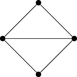
Find all \(8\) spanning trees of
the graph below.
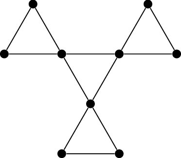
Let \(G\) be the graph shown
below:
Identify all the bridges in \(G\). (There should be \(5\).)
Find all the possible spanning trees of \(G\).
Prove that an \(n\)-vertex graph
with the degree sequence \(n-1, 1, 1, \dots,
1, 1\) must be a tree. What does such a graph look like?
Find a \(3\)-regular graph \(G\) which has a bridge. (You’ll need at
least \(10\) vertices.)
Let \(G\) be the graph shown
below:
Find a spanning tree \(T\) of
\(G\) whose diameter (the
largest distance between any two vertices, as defined in Chapter 5) is as large as
possible.
Is it possible to find two spanning trees of \(G\) that have only \(3\) edges in common? Give an example or
explain why it is not possible.
Let \(G\) be a \(4\)-regular graph in which edge \(xy\) is a bridge. Then \(G-xy\) should have a connected component
containing \(x\), and a connected
component containing \(y\). Describe
the degree sequences of each component.
Conclude that a \(4\)-regular
graph cannot have a bridge.
Prove that \(T\) is a tree if
and only if, between any two vertices of \(G\), there is exactly one path. (This is
another of the many characterizations of trees to accompany
Proposition 9.3 and Proposition 9.4.)
Theorem 9.5 assumes that all edges of the graph
have distinct costs: there are no ties.
Prove that if there are ties between the costs of some edges,
then we can still conclude one of two things in the proof: either we
find a spanning tree cheaper than \(T'\) (so \(T'\) cannot be the MCST) or \((T' + e) - e'\) is a spanning tree
with the same cost as \(T'\), but
“closer” to \(T\) in some
sense.
Explain why this is enough to still deduce that \(T\) is an MCST (even if it might not be
unique).
Use this to prove that every spanning tree of the cube graph
\(Q_3\) must have \(7\) edges. (Do not, of course, use my claim
that every spanning tree of \(Q_3\) is
isomorphic to one of the six trees in Figure 9.2.)