This chapter is an introduction to the ideas you’ll need to learn
about planar graphs. Most applications of graph theory to geometry are
based on Euler’s formula and the face length formula, which you will see
in this chapter.
The toughest decision for me in presenting this material was to
decide how much of the technical geometry to include. The truth is that
when working with planar graphs, we don’t want to, and also don’t have
to, worry about these details. The standard academic solution is to
begin with a section of technical preliminaries. However, this is also a
good way to bore all my readers before we get to the good part.
My compromise was to include rigorous technical proofs of the
geometric claims in the last section of this chapter, for the interested
reader only. Usually, I cite earlier theorems and lemmas in the textbook
when I use them, but in this case, I won’t, so that if you don’t want to
think about these details, you won’t have to. However, I have taken care
to make sure that every argument in this part of the textbook can be
made rigorous using one of the claims in this section.
Three utilities
Some puzzles are invented because they have a clever solution. Other
puzzles are invented because they have no solution; I suspect that
sometimes, the motivation is to keep a clever child quietly working on
the puzzle for a long time without worries that the child will actually
ever solve the puzzle and bother you again.
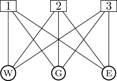
A classic entry in this genre of puzzles is the three utilities
problem [66]. Here,
three houses (which we will number \(1\), \(2\), and \(3\)) need to be provided water, gas, and
electricity by lines from three central utilities (which we will label
w, g, and
e). The required connections are shown in
Figure 21.1(a); however, this diagram is not
a solution because (for some reason that’s never been clear to me) water
lines, gas lines, and electricity lines cannot cross. Perhaps the
utility providers in this town have not yet learned about the third
dimension.
The utility graphNot a solutionA mandatory hexagon
The three utilities problem
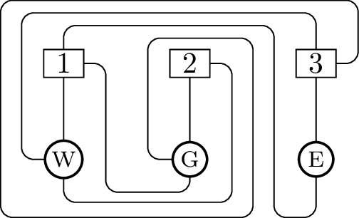
In any case, there is no way to solve the problem. Many attempts look
like the diagram in Figure 21.1(b); here, curved paths that
circle around each other in complicated ways may confuse even the solver
into forgetting that house 2 still does not have electricity. (The
inhabitants of house 2 are presumably very clear on this point,
however.)
But why do all attempts fail? Before presenting you with any general
theory, let me give a specific argument for the utility graph. (This is
not the most common argument, and [66] contains another simple solution. I
follow the same approach as West’s Introduction to Graph
Theory[104], and for
the same reason: it is a special case of the overlap graph technique we
will see in Chapter 22.)
The utility graph shown in Figure 21.1(a) is isomorphic to another
graph we have a name for; what is it?
We have a couple of names, actually! The
utility graph is isomorphic to the complete bipartite graph \(K_{3,3}\); it is also isomorphic to the
circulant graph \(\operatorname{Ci}_6(1,3)\).
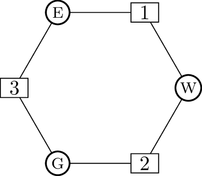
The utility graph is Hamiltonian; one possible Hamilton cycle is
represented by \[(1, \text{\scriptsize W}, 2,
\text{\scriptsize G}, 3, \text{\scriptsize E}, 1).\] No matter how this cycle is
drawn in a hypothetical solution, it will be a closed loop in the plane
with an inside and an outside. (This is even true in Figure 21.1(b), though the closed loop
is rather complicated!) To help us visualize the closed loop, I will
draw it as a regular hexagon in Figure 21.1(c),
though of course the loop doesn’t have to look anything like this.
There are still three edges that we have not drawn: the edges \(1\text{\scriptsize G}\), \(2\text{\scriptsize E}\), and \(3\text{\scriptsize W}\). Only one of these edges can
be drawn inside the loop. For example, if we draw edge \(1\text{\scriptsize G}\) inside the loop, then it
separates vertices \(2\) and \(\text{\scriptsize W}\) from vertices \(3\) and \(\text{\scriptsize E}\), so neither \(2\text{\scriptsize E}\) nor \(3\text{\scriptsize W}\) can also be drawn inside the
loop.
Of course, we can still draw either of those edges outside the loop.
However, an identical problem occurs there. Suppose we decide to draw
edge \(2\text{\scriptsize E}\) outside the loop.
No matter how we do it, the edge and the loop divide the outside into
two pieces: one (call this \(F_1\))
bounded by the edges \(\{2\text{\scriptsize E},
2\text{\scriptsize G}, 3\text{\scriptsize E}, 3\text{\scriptsize G}\}\) and one (call this
\(F_2\)) bounded by the edges \(\{1\text{\scriptsize E}, 1\text{\scriptsize W}, 2\text{\scriptsize E},
2\text{\scriptsize W}\}\). One of these pieces will be finite and the other
infinite, but that doesn’t concern us in any way.
What does concern us is that once we’ve drawn edge \(2\text{\scriptsize E}\) outside the loop, we can’t do
the same thing with edge \(1\text{\scriptsize G}\) or \(3\text{\scriptsize W}\). A curve in the plane from
\(1\) to \(\text{\scriptsize G}\) drawn outside the loop, for
example, would start in \(F_1\) and end
in \(F_2\), so at some point it would
have to cross one of the boundaries.
Of course, neither drawing \(1\text{\scriptsize G}\) inside the loop nor drawing
\(2\text{\scriptsize E}\) outside the loop is
required, but we’re stuck no matter what we try: the loop has two sides
(inside and outside) and each side only has room for one edge, but we
have three edges left to draw. Because \(3>2\), the three utilities problem has
no solution.
Planar graphs
The three utilities problem is one special case of a general problem
in graph theory: which graphs can be drawn in the plane without
crossings?
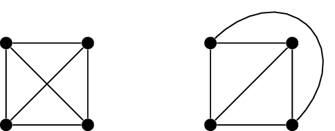
Sometimes answering this question is easy. For example, Figure 21.2(a) shows two ways to draw the
complete graph \(K_4\). In the standard
one, the two diagonal edges cross; however, we can draw one of the two
edges differently and eliminate that crossing.
Two drawings of \(K_4\)Which graph is planar?
Planar and non-planar graphs
Sometimes answering this question is hard. Both of the graphs in
Figure 21.2(b) are drawn with many
crossing edges. For one of them, this can be fixed; for the other, there
is no way to avoid crossings. However, it is far from obvious which
graph has which property; we will need to learn more before we answer
this question.
In Figure 21.2(a), we
avoid crossings by curving one of the edges. However, we can also draw
\(K_4\) in the plane with \(6\) straight edges that don’t cross;
how?
Put \(3\)
vertices of \(K_4\) at the corners of a
triangle, and put the \(4\)th vertex inside the
triangle.
It’s important to distinguish between two similar concepts: “a graph
that can be drawn in the plane with no crossings” and “a drawing of a
graph in the plane with no crossings.” The first of these is a graph
invariant. If \(G\) and \(H\) are two isomorphic graphs, and we can
draw \(G\) in the plane with no
crossings, then we can draw \(H\) in
the plane with no crossings: just relabel the drawing of \(G\).
However, whether or not a graph is drawn with no crossings is not a
graph invariant! Figure 21.2(a)
makes this clear: the graph \(K_4\) can
be drawn with crossings, but it can also be drawn without crossings,
without changing the graph itself.
Accordingly, we have two definitions to separate these concepts.
Definition 21.1. A plane
embedding of a graph \(G\) is
a drawing of \(G\) in the plane with no
crossings.
A planar graph is a graph that has a plane
embedding.
This means that our discussion of the the three utilities problem can
be taken as a proof of the following proposition:
Proposition 21.1. The complete bipartite graph
\(K_{3,3}\) is not planar.
Let me emphasize again that a planar graph and a plane embedding are
two different things. A planar graph is still just an abstract object: a
set of vertices and a set of edges. We haven’t picked a particular
drawing for it, and there could be many drawings that are different from
each other in important ways.
When using the assumption that a graph \(G\) is planar in a proof, we should usually
begin by choosing a plane embedding of \(G\). However, we should be careful when
talking about properties of that plane embedding: they are not
properties of the graph \(G\) itself,
unless we can prove that all plane embeddings of \(G\) share those properties. In this
chapter, we will see some examples where we can prove this, and some
examples where we can’t.
We will occasionally have reason to talk about plane embeddings of
multigraphs, rather than graphs. This will not come up when deciding if
a graph is planar or not: a multigraph is planar if and only if its
simplification is planar. But we sometimes want to consider plane
embeddings of multigraphs as objects of study in their own right.
Faces
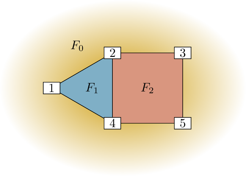
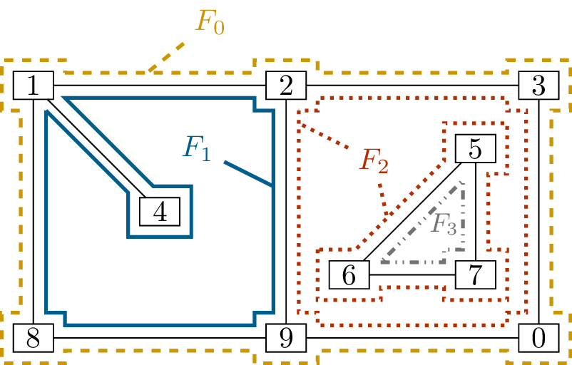
The diagrams in Figure 21.3 show two plane embeddings in which
I’ve highlighted several regions of the plane. (The shading in regions
that I’ve labeled \(F_0\) in both
diagrams is meant to indicate that they are infinite regions, extending
outward to the rest of the plane.) We call these the faces of the plane
embedding.
Definition 21.2. The faces of a
plane embedding are the connected regions of the plane separated by the
edges of the plane embedding. One of the faces is infinite, and contains
all points sufficiently far from the plane embedding; it is called the
outer face.
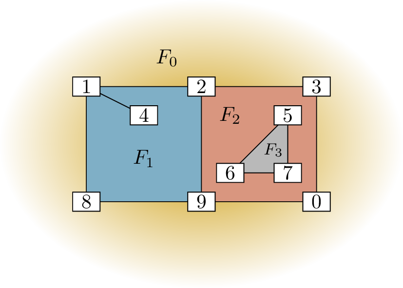
Simple facesMore unusual faces
Examples of faces in plane embeddings
Faces are the link between the geometry of a plane embedding and the
abstract structure of the graph \(G\).
In the graph \(G\) itself, a region of
points does not exist. So what does? What’s left is the boundary of the
face: the vertices and edges that separate it from the other faces.
In ideal circumstances, the boundary of a face is a cycle, in which
case (as usual) it is represented by a closed walk. Don’t forget that
the cycle doesn’t have a prescribed starting point or direction, so it
can be represented by many different closed walks.
In Figure 21.3(a),
which closed walks represent the boundary of the faces?
The boundary of \(F_1\) is represented by \((1,2,4,1)\), the boundary of \(F_2\) is represented by \((2,3,5,4,2)\), and the boundary of \(F_0\) is represented by \((1,4,5,3,2,1)\).
However, the boundary of a face is not always as nice. In Figure 21.3(b), the boundaries of faces \(F_1\) and \(F_2\) are a bit more unusual:
In the case of \(F_1\), we would
like edge \(14\) to be taken into
account, even though it only separates face \(F_1\) from itself, so the boundary is not a
cycle. However, the closed walk \((1,2,9,8,1,4,1)\) still seems to represent
the boundary.
In the case of \(F_2\), the
boundary is not even connected! We need two closed walks: \((2,3,0,9,2)\) and \((5,6,7,5)\).
In general, the boundary of a face is represented by one or more
boundary walks. A boundary walk is found by starting at
any vertex on the boundary of the face, and following edges out of it in
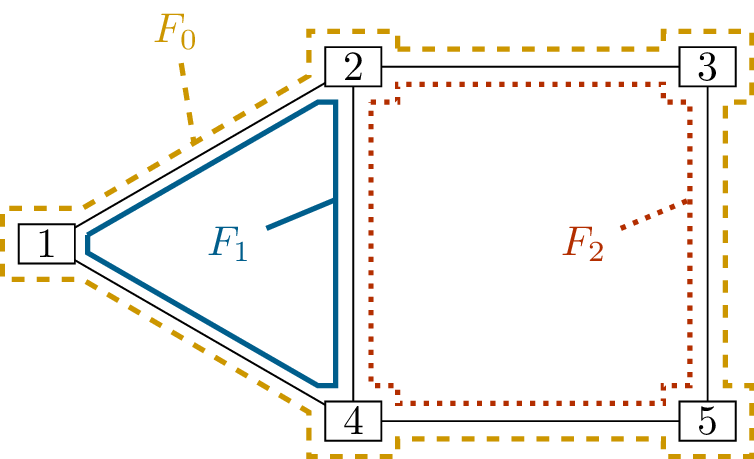
some direction, while staying inside the face. Figure 21.4 shows the boundary walks of
the faces of the two example graphs we looked at.
Simple facesMore unusual faces
Boundary walks of the faces in Figure 21.3Looking at Figure 21.3(b), why does face \(F_2\) have two boundary walks?
The graph has multiple connected
components, each of which contributes a boundary walk to \(F_2\).
Why is edge \(14\) in Figure 21.3(b) on
the boundary walk of \(F_1\)
twice?
The same face, \(F_1\), is on both sides of the edge.
Every edge \(xy\) is either on two
boundary walks of two different faces, or on the boundary walk of the
same face twice. The difference between these two cases comes down to
the following test:
Lemma 21.2. If edge \(xy\) is a bridge of planar graph \(G\), then in every plane embedding of \(G\), it appears on the boundary walk of the
same face twice.
If edge \(xy\) is not a bridge,
then in every plane embedding of \(G\),
it separates two faces, and appears once on the boundary walk of each
face.
Proof. If the same face \(F\) is on both sides of edge \(xy\) when it is drawn in the plane
embedding, then we can draw a curve from one side of \(xy\) to the other while always staying
inside \(F\). If \(xy\) is deleted, we can complete that curve
to a closed loop drawn entirely inside \(F\). Of the two vertices \(x\) and \(y\), one is drawn inside that closed loop
and the other outside it, and no edges cross the loop; therefore there
is no way to get from \(x\) to \(y\). This makes \(xy\) a bridge.
If edge \(xy\) separates two faces
\(F_1\) and \(F_2\), then each of them has a boundary
walk using edge \(xy\) once. Without
loss of generality, such a boundary walk goes from \(x\) to \(y\), and returns along some \(y-x\) walk without using edge \(xy\) again: that walk exists in \(G-xy\). Every \(y-x\) walk contains a \(y-x\) path (by Theorem 3.1), so there is
an \(x-y\) path in \(G-xy\). This means that in \(G\), there is a cycle containing \(xy\), so \(xy\) is not a bridge.
The above arguments tell us whether \(xy\) is a bridge or not based on what it
does in one plane embedding. But regardless of the plane embedding, edge
\(xy\) either is a bridge in graph
\(G\) or it isn’t, so it must have the
same behavior in every plane embedding. ◻
The most important property of the boundary of a face is its length.
The length of a face \(F\), written \(\operatorname{len}(F)\), is the sum of the
lengths of boundary walks of \(F\).
Equivalently, \(\operatorname{len}(F)\)
is the number of edges on the boundary of \(F\), counting an edge twice if it is not on
the boundary of any other face.
When we give the definition of \(\operatorname{len}(F)\) in its second form,
it seems unnatural and artificial, though you may remember that when we
defined the degree of a vertex of a multigraph in Chapter 7, we did something
similar. Just like back then, it is all in service of making sure a nice
lemma holds in all possible cases:
Lemma 21.3 (Face length formula). If \(G\) is a planar graph with \(m\) edges, and a plane embedding of \(G\) has faces \(F_0, F_1, \dots, F_{r-1}\), then \[\sum_{i=0}^{r-1} \operatorname{len}(F_i) =
2m.\]
Proof. Each edge of \(G\)
appears once on boundary walks of two faces, or twice on the boundary
walks of one face. In either case, it contributes \(+2\) to the sum of face lengths, so the
contributions of all \(m\) edges add up
to \(2m\). ◻
The face length formula tells us that the sum of the lengths of the
faces does not depend on the plane embedding chosen. (After all, it is
equal to \(2m\), which certainly cannot
change based on the plane embedding!) The individual lengths, however,
certainly do depend on the embedding!
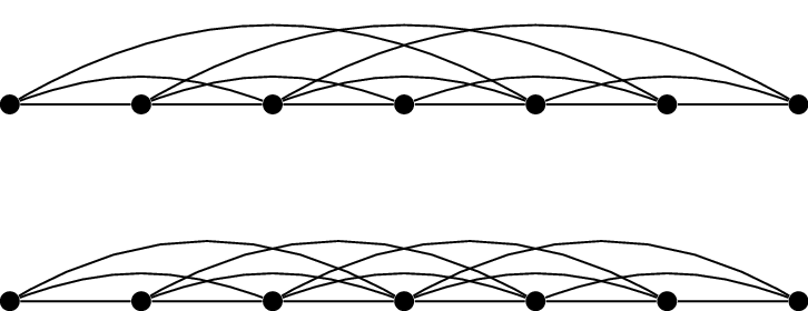
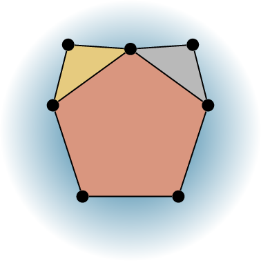
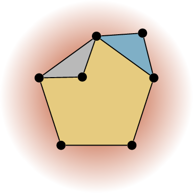
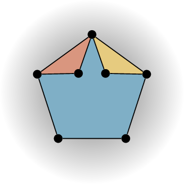
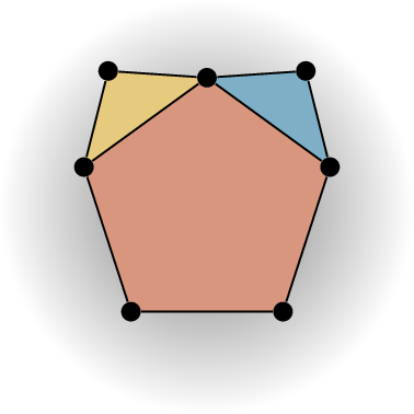
Three embeddings of the same graph
Figure 21.5 shows three different
plane embeddings of the same \(7\)-vertex graph. (I have deliberately not
used consistent colors to discourage you from the temptation of feeling
that the faces of one embedding correspond in any way to the faces of
another.) However, the face lengths vary:
The embedding in Figure 21.5(a) has
two faces of length \(3\), one face of
length \(5\), and an outer face of
length \(7\).
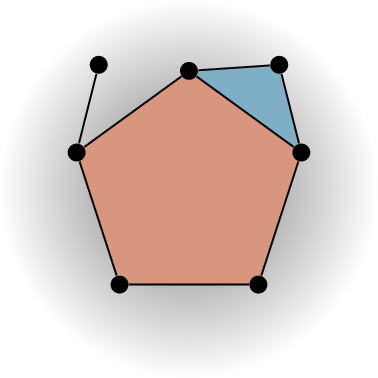
The embedding in Figure 21.5(b) has
two faces of length \(3\), and two
faces (including the outer face) of length \(6\).
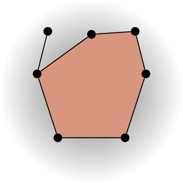
The embedding in Figure 21.5(c) is
almost like the one in Figure 21.5(a): it
also has faces of lengths \(3, 3, 5,
7\). However, in this case, the embedding of length \(5\) is the outer face.
Euler’s formula
The face length formula is one of two important identities regarding
the faces of a plane embedding. The other one is Euler’s formula (one of
several mathematical statements by that name!), which helps us count the
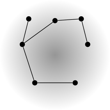
faces in a plane embedding. You may have noticed that no matter how hard
we tried to find different plane embeddings in Figure 21.5,all of them had four
faces. This is not a coincidence, and it will follow from Euler’s
formula that the number of faces in a plane embedding depends only on
the graph.
Theorem 21.4 bears Euler’s name because he
was the first to look at the problem in a general case [32]. Euler did not consider
the problem for planar graphs, but for polyhedra, which we will study in
Chapter 23. Many other
mathematicians later approached the formula from different directions;
see [27] for a
brief history, as well as further references and many different
proofs.
Euler’s formula is often stated as \(V-E+F=2\), where \(V\) is the number of vertices, \(E\) is the number of edges, and \(F\) is the number of faces. I can’t bring
myself to do this, since I think of \(V\) and \(E\) as sets, not numbers. In graph theory,
\(n\) and \(m\) are the standard variables to use when
you want to count the vertices and edges in a graph, respectively. There
is no standard variable for faces, so I will use \(r\) (for “region”). Meanwhile, \(k\) will be our variable of choice for
connected components, as it already was in Chapter 10.
Theorem 21.4 (Euler’s formula). If a connected
plane embedding (of a graph or a multigraph) has \(n\) vertices, \(m\) edges, and \(r\) faces, then \[n - m + r = 2.\] In general, if there are
\(k\) connected components, this
formula becomes \[n - m + r - k =
1.\]
Proof. We induct on the number of edges, \(m\). Since removing an edge from a graph
may disconnect it, we should work directly with the second, more general
form of Euler’s formula; the first form will follow by setting \(k=1\).
Our base case is \(m=0\). Here,
\(n\) (the number of vertices) is equal
to \(k\) (the number of connected
components), and there is only one face: \(r=1\). So \(n - m
+ r - k\) starts out at \(1\).
Now assume for some \(m\ge 1\) that
Euler’s formula holds for all plane embeddings with \(m-1\) edges, and consider a plane embedding
of a graph \(G\) with \(m\) edges. We will arbitrarily pick an edge
\(xy\) to delete.
How can the deletion of edge \(xy\) affect \(n\), \(m\), \(r\), and \(k\)?
It never affects \(n\), and always decreases \(m\) by \(1\).
It may decrease \(r\) by \(1\), if \(xy\) previously separated two faces.
It may increase \(k\) by \(1\), if \(xy\) was the only way to get from \(x\) to \(y\).
We would like \(n - m + r - k\) to
stay the same, so we would like exactly one one of two things to happen:
either \(r\) decreases by \(1\), or \(k\) increases by \(1\), but not both.
Fortunately, this is exactly what Lemma 21.2 tells us! If edge \(xy\) is a bridge, its deletion increases
\(k\) by \(1\); however, in every plane embedding, the
same face is on both sides of \(xy\),
so \(r\) stays the same. If edge \(xy\) is not a bridge, then it separates two
faces, so deleting it decreases \(r\)
by \(1\); however, it is not a bridge
so its deletion does not affect \(r\).
In summary: the number of vertices, edges, faces, and components in
the plane embedding of \(G-xy\), which
we’ll denote \((n', m', r',
k')\), is either \((n, m-1, r-1,
k)\) or \((n, m-1, r, k+1)\). By
the induction hypothesis, \(n' - m' +
r' - k' = 1\), which tells us either that \(n - (m-1) + (r-1) - k = 1\) or that \(n - (m-1) + r - (k+1) = 1\); both of these
simplify to \(n - m + r - k = 1\).
How the triple \((n,m,r)\)
changes as we erase edges in a plane embedding
By induction, the formula holds for all plane embeddings. You can see
the induction in action in Figure 21.6.
Here, we’ve chosen to delete only edges that keep the graph connected,
so going from Figure 21.6(a) to Figure 21.6(d), \(r\) decreases at each step while \(k\) remains equal to \(1\). At this point, if we delete more
edges, it will decrease \(m\) and
increase \(k\) while keeping \(n\) and \(r\) the same. ◻
In Euler’s formula, the variables \(n\), \(m\), and \(k\) are properties of the graph \(G\), while \(r\) is computed from a specific plane
embedding. However, we can solve for \(r\) in terms of \(n\), \(m\), and \(k\): it is \(m -
n + k + 1\), or just \(m-n+2\)
if \(G\) is connected.
How can these observations be
reconciled?
It means that although different plane
embeddings can have faces with different shapes and with different
lengths, two plane embeddings of the same graph are guaranteed to have
the same number of faces: the number predicted by Euler’s formula.
We should still avoid talking about “the faces of \(G\)”, because that is not a well-defined
concept, as Figure 21.5
shows. Talking about the number of faces that \(G\) has is also incorrect, but if you said
it to my face, I would only disapprove a little; after all, if we pick
different embeddings, we will still not disagree about the number of
faces.
Barycentric subdivisions
Euler’s formula and the face length formula have applications to
geometry in scenarios where the problem can be modeled as a graph. To
illustrate this, let me tell you about a problem that once misled me
until I thought of applying Euler’s formula to solve it.
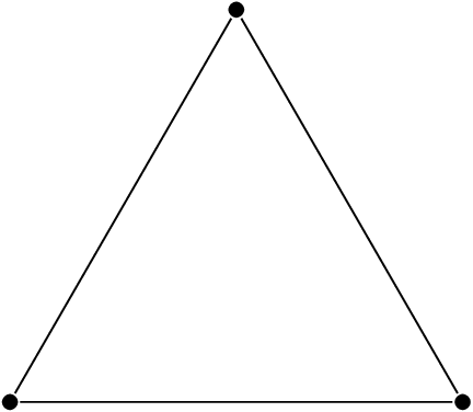
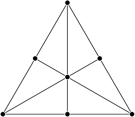
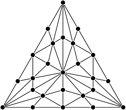
The barycentric subdivision of a triangle subdivides it into
six triangles, by drawing the three medians: the lines connecting each
corner of the triangle to the midpoint of the opposite sides. (The three
lines in this way always intersect at a single point, which is called
the centroid of the triangle.) An example is shown in Figure 21.7(b), though the triangle we start with
does not have to be equilateral.
Stage 0Stage 1Stage 2
Iterated barycentric subdivisions
We can iterate this process: start with the barycentric subdivision
of a triangle, and then take the barycentric subdivision of each of the
six small triangles that result. This is shown in Figure 21.7(c), but we don’t have to stop there; we
can keep going, by taking the barycentric subdivision of each of the
\(36\) small triangles in that diagram.
Let’s say that stage \(n\) of this
process is the result we get when we apply the operation “take the
barycentric subdivision of every triangle which does not have any
smaller triangles inside it” \(n\)
times.
I was interested in the number of vertices in this diagram: I placed
a vertex at every point where two or more segments met, or in other
words, at every point which is the corner of one or more triangles. If
you count the vertices in Figure 21.7, you
get \(3\) vertices in Figure 21.7(a), \(7\) vertices in Figure 21.7(b), and \(25\) vertices in Figure 21.7(c). I went one step further and
laboriously computed the number of vertices in Stage 3, which turned out
to be \(121\).
I did not even want to think about drawing Stage 4, so my next step
was to go to the Online Encyclopedia of Integer Sequences and search for
the sequence \(3, 7, 25, 121\). At the
time, there was essentially one candidate formula in the search results
(plus a few minor variants which were clearly wrong for this problem),
but it was a very nice formula: it suggested that the \(n\)th stage would contain \((n+2)! + 1\) vertices.
At this point, there is a quick way to see
that this formula can’t possibly be right for all \(n\), because the number of vertices grows
at most exponentially. Why?
The number of triangles in the subdivision
is much easier to count: it is \(6^n\)
in the \(n\)th stage,
because each triangle gets subdivided into six triangles. Each triangle
has \(3\) corners, giving \(3 \cdot 6^n\) vertices total. This counts
some vertices many times, because some vertices are the corners of many
triangles; however, it counts each vertex at least once, so there are at
most \(3\cdot 6^n\) vertices.
Unfortunately, I only thought of this quick way later. At the time, I
spent a while trying to prove the formula \((n+1)!+1\) combinatorially. Maybe we should
label the vertices with permutations of \(n+2\) elements, but leave the central
vertex unlabeled? In the end, it occurred to me to try Euler’s formula,
and that’s when my house of cards fell apart.
Why Euler’s formula? Well, the diagrams shown in Figure 21.7 and the ones that come after
are all plane embeddings: the vertices are exactly as I have defined
them already, and the edges are the line segments connecting the
vertices. We can hope that the edges and faces will be easier to count
than the vertices, replacing one hard counting problem with two easier
ones.
In this case, to apply Euler’s formula, we should start with the
faces. It is not quite true that there are \(6^n\) faces, all with \(3\) sides, because there is also an outer
face; there are \(6^n + 1\) faces
total.
What is the length of the outer face?
It is \(3 \cdot
2^n\): in the \(n\)th
stage, each side of the triangle has been divided into \(2^n\) segments, which are all edges of the
plane embedding.
How can we find the number of edges?
We can add up the lengths of the faces and
apply the face length formula.
With \(6^n\) faces of length \(3\) and one face of length \(3 \cdot 2^n\), the sum of face lengths is
\(3 \cdot 6^n + 3 \cdot 2^n\), so there
\(\frac{3\cdot 6^n + 3 \cdot 2^n}{2}\)
edges. Solving for the number of vertices in Euler’s formula, we get
\[\frac{3\cdot 6^n + 3 \cdot 2^n}{2} - (6^n +
1) + 2,\] which simplifies to \(\frac{6^n + 3 \cdot 2^n}{2} + 1\). When
\(n=4\), the first case I did not
consider, this formula tells us that there are \(673\) vertices. This is the first time the
true answer disagrees with the incorrect formula \((n+2)! + 1\) (which gives \(721\)).
This story has a happy ending, of sorts. Future mathematicians who
stumble upon this problem will not have the experience I did, because
the correct answer now also shows up in the OEIS: as sequence
A380996 [81].
Technical details
This section contains all the geometric arguments that we will need,
in this part of the textbook, to confirm our intuition about how planar
graphs can, and cannot be drawn. Though I will not cite specific claims,
I have made sure that every geometric fact we need is contained
somewhere in this section.
First of all, we should be more precise about what a plane embedding
exactly is. There is not much to say about vertices: every vertex is
drawn as a point in the plane. An edge should be drawn as some path
between its two endpoints; two edges do not contain any common interior
points, and in particular their interiors do not pass through any
vertices. But what kind of paths should we allow?
In principle, any kind of continuous simple curve will do: the image
of a continuous injective function \(f\colon
[0,1] \to \mathbb R^2\), where the points \(f(0)\) and \(f(1)\) are the two endpoints of the edge.
However, studying such things will drown us in a sea of topology for no
practical benefit.
It is sufficient to consider edges which are polygonal
curves: made up of finitely many line segments joined end to end
(and not intersecting otherwise). In a closed polygonal curve, or
polygon, the last line segment ends where the first segment
starts. Polygonal curves and polygons can approximate any crazier shape
arbitrarily well; you won’t be able to tell the difference. Practically
speaking, when you encounter a planar graph (for example, derived from a
map specified by latitude and longitude coordinates), it will already
have edges in this form. Paths and cycles in a planar graph also become
polygonal curves and polygons, respectively, in a plane embedding.
To define faces in a plane embedding, we want to be able to tell
which points are in the same connected region of the plane (separated by
the edges). Our test for this also uses polygonal curves: two points
\(x\) and \(y\) are in the same face if there is a
polygonal curve from \(x\) to \(y\) that does not intersect the plane
embedding.
Why is this notion of connectedness
practically useful to us?
It tells us which new edges we could add
to the plane embedding, because the edges are also polygonal
curves.
There are a few more things to say about this notion of
connectedness. From the point of view of theory, the most fundamental is
the Jordan curve theorem, which states an obvious-seeming fact: every
polygon separates the plane into exactly two connected regions, an
inside and an outside, with the polygon as their boundary. (That is,
points on the polygon are exactly the points arbitrarily close to both
the inside and the outside.) The Jordan curve theorem holds for all
continuous curves, not just polygons, but even in the polygonal case it
is not easy to prove; I will skip it, to avoid too lengthy a geometric
detour.
From the point of view of algorithms, it is not that interesting to
know merely that every polygon has an inside and an outside; we would
like to know what they are! A standard test for this is the ray casting
algorithm: given a point \(x\) and a
polygon \(P\), draw an infinite ray (or
half-line) starting at \(x\). Then
\(x\) is inside \(P\) if the ray crosses \(P\) an odd number of times, and outside
\(P\) if the ray crosses \(P\) an even number of times.
The choice of ray doesn’t matter, and in programming applications,
it’s often fine to take a horizontal or vertical ray, for simplicity. We
do run into some technicalities if the ray passes through a corner of
\(P\) or contains an entire line
segment of \(P\). It’s possible to make
sense of this situation: we say that if a segment of \(P\) has an endpoint on the ray, that
segment crosses the ray if it lies to the left of the ray, but not if it
lies to the right. But this is very technical, and it’s easier to avoid
it if possible.
We can get a more general test as a consequence of this
algorithm:
Claim 21.5. Let \(P\) be a polygon, and let points \(x\) and \(y\) be connected by a polygonal curve whose
segments never start or end on \(P\),
and never intersect a segment of \(P\)
in a sub-segment, only in a point.
Then \(x\) and \(y\) are on the same side of \(P\) if and only if the polygonal curve
connecting them crosses \(P\) an even
number of times.
Proof. We can subdivide the \(x-y\) polygonal curve into segments that
each cross \(P\) at most once. If a
segment crosses \(P\) once, its
endpoints are on opposite sides: this is verified by the ray casting
algorithm with a ray parallel to the segment, starting at either
endpoint. So with every crossing, the polygonal curve switches to a
different side of \(P\).
Since there are only two sides, the polygonal curve ends on the same
side as it started if and only if it switched sides an even number of
times. ◻
We can now easily test which points lie in the same face, but do not
have an easy definition of the boundary of a face. To obtain it, we need
a geometric understanding of boundary walks.
Given a plane embedding, pick a value \(\varepsilon>0\) much smaller than every
distance between a line segment and an endpoint of another end segment.
Then surround every line segment by a thin rectangular loop: if the line
segment has length \(\ell\), draw a
\(2\varepsilon \times (\ell +
2\varepsilon)\) rectangle with the line segment at its center.
Orient each of these loops counterclockwise.
To find a boundary walk containing a particular segment, start going
around its thin rectangular loop on either of the long sides. If this
trajectory hits the loop around a different line segment (which only
happens near the end of the segment), switch to following that loop.
Keep going like this until this trajectory returns where it started (as
it must, because we only have finitely many segments).
The result is a polygon that never crosses the plane embedding. It
also stays within distance \(\varepsilon\) of a walk in the planar
graph: it can only switch from following one edge to following another a
vertex they share, because it never gets close enough to another edge
anywhere else. We say that this walk is a boundary walk in the graph,
and the polygon is the corresponding boundary walk in the plane
embedding. Although boundary walks do not always represent cycles, we
still consider two boundary walks to be the same if one is a shifted
and/or reversed version of another.
The following is immediate from the definition.
Each edge either lies on one boundary walk twice, or on two
boundary walks, since each thin rectangular loop has two long
sides.
Each boundary walk in the plane embedding is contained entirely
in one face, and we say it is a boundary walk of that face; a face can
have multiple boundary walks.
Let \(xy\) be an edge of a planar
graph \(G\), and let \(C\) be the polygonal curve representing
\(xy\) in a plane embedding of \(G\). Many times, such as in the proof of
Euler’s formula, we want to understand edge \(xy\) by comparing the plane embedding of
\(G\) and the plane embedding of \(G-xy\) obtained by erasing \(C\). In that second plane embedding, \(C\) stays entirely in some face \(F\), because \(C\) does not cross any other edge. The
following claim is a more careful formal proof of Lemma 21.2.
Claim 21.6. Either \(F-C\) is a single face in the plane
embedding of \(G\), \(xy\) lies on its boundary walk twice, and
\(xy\) is a bridge of \(G\); or \(F-C\) is the union of two faces in the
plane embedding of \(G\), \(xy\) lies on each of their boundary walks
once, and \(xy\) is not a bridge of
\(G\).
Proof. Starting from either side of a segment of \(C\), construct boundary walks using \(xy\), letting \(B_1\) and \(B_2\) be the corresponding polygons in the
plane embedding; possibly, \(B_1=B_2\).
If \(B_1 = B_2\), then follow this
polygon from one side of \(C\) to a
point \(2\varepsilon\) away on the
other side, and connect by cutting across \(C\). The result is a polygon \(P\) that only crosses \(C\), and only once. No edge of \(G-xy\) crosses \(P\), and \(x\) and \(y\) are on opposite sides (because \(C\) crosses \(P\) once), so there is no \(x-y\) path in \(G-xy\): \(xy\) is a bridge. If \(B_1 \ne B_2\), then each boundary walk in
\(G\) uses edge \(xy\) only once, so it also contains an
\(x-y\) path in \(G-xy\), proving that \(xy\) is not a bridge.
Each point \(z\in F-C\) can be
joined to a point of \(C\) by a
polygonal curve not crossing the plane embedding of \(G-xy\); before it touches \(C\), it must cross either \(B_1\) or \(B_2\). So all points of \(F-C\) are in the face containing \(B_1\) or the face containing \(B_2\). (The exception is points within
\(\varepsilon\) of \(C\), which can reach \(B_1\) or \(B_2\) by taking a step of length at most
\(\varepsilon\) away from \(C\).) So there are at most \(2\) faces, and if \(B_1 = B_2\), there is only one face.
Conversely, if \(F-C\) is a single
face in the plane embedding of \(G\),
then take a line segment of length \(2\varepsilon\) from \(B_1\) to \(B_2\) that cuts across \(C\); its endpoints are both in \(F-C\), so this line segment can be
completed to a polygon \(P\) that does
not cross the plane embedding of \(G\)
again. As before, no edge of \(G-xy\)
crosses \(P\), and \(x\) and \(y\) are on opposite sides (because \(C\) crosses \(P\) once), so there is no \(x-y\) path in \(G-xy\): \(xy\) is a bridge. ◻
The machinery we’ve built so far is enough to prove Euler’s formula.
As a special case, consider a planar graph \(G\) with no cycles: a forest. With \(n\) vertices and \(k\) connected components, the forest has
\(n-k\) edges, by Theorem 10.1. Substituting this into Euler’s
formula, we learn that the forest only has one face.
With at least two faces, the picture changes:
Claim 21.7. If a plane embedding of \(G\) has at least two faces, then some
boundary walk of every face contains a cycle.
Proof. Let \(F\) be any
face; since it is not the only face, we can pick a point \(p \in F\) and a point \(q \notin F\). The line segment \(pq\) leaves \(F\), so at some point it must cross an edge
\(xy\) on a boundary walk of \(F\) to do so. Replace \(pq\) by a short sub-segment, if necessary,
to ensure that \(pq\) only crosses
\(xy\) once, and does not cross any
other edge of the plane embedding.
In the plane embedding of \(G-xy\),
points \(p\) and \(q\) are part of the same face (since \(pq\) no longer crosses any edge). By
Claim 21.6, the boundary walk of \(F\) using \(xy\) only uses it once: after going from
\(x\) to \(y\), it is a \(y-x\) walk that does not use edge \(xy\). That \(y-x\) walk contains a \(y-x\) path, which together with edge \(xy\) becomes a cycle. ◻
So far, we’ve been using the geometry of polygons to understand plane
embeddings, but we can do this in reverse, as well.
Claim 21.8. If \(p\) and \(q\) are two points on a polygon, then a
polygonal curve that joins \(p\) and
\(q\) divides one side of the polygon
into two connected regions.
Proof. Here, we think of the polygon plus the curve joining
\(p\) and \(q\) as a plane embedding of a cycle graph
with an extra edge (whose endpoints are drawn at \(p\) and \(q\)). That extra edge falls under the
second case of Claim 21.6,
proving the claim. ◻
Claim 21.9. If \(p\), \(q\), \(r\), and \(s\) are four points appearing on a polygon
\(P\) in that order, then a polygonal
curve joining \(p\) and \(r\) cannot be drawn on the same side of the
polygon as a polygonal curve joining \(q\) and \(s\) without crossing it.
Proof. Suppose such a diagram existed; then it would be an
embedding of \(K_4\), with vertices
placed at \(p\), \(q\), \(r\), and \(s\). Such an embedding does exist: \(K_4\) is a planar graph. But it cannot have
the shape it needs to have here!
By Euler’s formula, there are \(4\)
faces total (\(4-6+4=2\)). One face of
the plane embedding is the side \(P\)
containing neither of the added curves; it has length \(4\). We know less about the others, but by
Claim 21.7 each contains a cycle, so
has length at least \(3\). The sum of
the face lengths is at least \(4+3+3+3=13\), but it must also be \(12\) by the face length formula, which is a
contradiction. Therefore the diagram we started with cannot exist. ◻
There is one final claim that we will need to construct new plane
embeddings of graphs:
Going from a plane embedding of \(G\) to a plane embedding of \(G \bullet e\) in Chapter 22;
Finding the dual graph of a plane embedding in Chapter 23;
Finding a plane embedding of the graph of adjacencies of a map in
Chapter 24.
Claim 21.10. Given a plane embedding with a face
\(F\), a point \(p \in F\), and points \(q_1, q_2, \dots, q_k\) on the boundary of
\(F\), it is possible to draw polygonal
curves from \(p\) to each of \(q_1, \dots, q_k\) that don’t cross each
other or the boundary of \(F\) (and
therefore stay inside \(F\)).
Proof. We will draw the polygonal curves one at a time.
First, draw a polygonal curve from \(p\) to a point on the same boundary walk as
\(q_1\) (which is possible by
definition of both points being in \(F\)). Then, follow that boundary walk until
its closest approach to \(q_1\), and
end with a straight line segment.
(It is useful to observe that that last line segment can never
intersect any part of the plane embedding: it is entirely contained in
one of the rectangular loops around a segment of an edge, which is too
close to that segment to touch any other segments.)
Once this is done, we can think of the result as a bigger plane
embedding where the point \(p\) and the
polygonal curve we drew are part of the boundary of a face \(F'\) contained in \(F\). We add another polygonal curve by
taking a short step out to the point \(p'\) on the boundary walk nearest \(p\), then drawing a polygonal curve from
\(p'\) to the next \(q_i\) in the same manner as before.
In general, this process can divide \(F'\) into two faces, and it’s not
guaranteed that the remaining points among \(q_1, q_2, \dots, q_k\) are all on the
boundary of the same one. However, if this happens, then \(p\) is on the boundary of both of them,
because the polygonal curve we drew from \(p\) is on the boundary of both, and we can
repeat on each of the faces formed separately. ◻
Practice problems
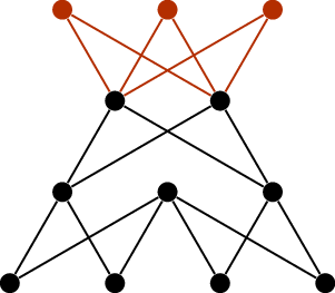
Find a plane embedding of the volcano graph, shown
below.
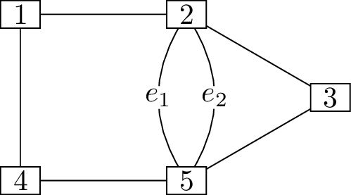
Consider the following planar multigraph:
Draw the following plane embeddings:
One where the outer face has length \(3\), with vertices \(2, 3, 5\) and edge \(e_1\) on its boundary, and the other faces
have lengths \(2\), \(4\), and \(5\).
One where the outer face has length \(4\), with vertices \(1, 2, 4, 5\) and \(e_1\) on its boundary, and the other faces
have lengths \(3\), \(3\), and \(4\).
One where the outer face has length \(2\), with edges \(e_1\) and \(e_2\) on its boundary.
Let \(G\) be a connected planar
graph. Suppose that a plane embedding of \(G\) has \(r\) faces, all of length \(4\).
Use the face length formula to find the number of edges of \(G\) (in terms of \(r\)).
Use Euler’s formula to find the number of vertices of \(G\) (in terms of \(r\)).
Can you find such a graph for \(r=8\)? What about for \(r=10\)?
Use an argument similar to the proof of Proposition 21.1 to show that the
complete graph \(K_5\) is not planar.
Start with a Hamilton cycle in \(K_5\),
then reason about where the remaining \(5\) edges can go.
Prove that all trees are planar graphs. Moreover, show that any
tree has a plane embedding in which all the edges are straight
lines.
(Hint: use induction. You’ll need to show that if \(x\) is a leaf of \(T\), then a plane embedding of \(T-x\) can be extended to a plane embedding
of \(T\).)
Here is another deceptive problem whose real solution can be
found with Euler’s formula. (It is documented along with many deceptive
patterns in “The Strong Law of Small Numbers” by Richard Guy [44].)
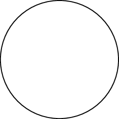
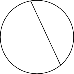
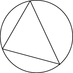
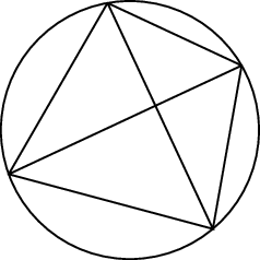
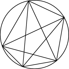
Put \(n\) points around a circle in
random positions (not equally spaced) and draw all \(\binom n2\) chords between those points;
wiggle the \(n\) points around, if
necessary, until no intersection point inside the circle lies on three
or more chords.
In the examples above (where \(n=1, 2, 3,
4, 5\)) the chords divide the circle into \(1\), \(2\), \(4\), \(8\), and \(16\) pieces, so you might be forgiven for
thinking that the number for general \(n\) is \(2^{n-1}\); it’s not! Use Euler’s formula to
find the correct answer.
Let \(G\) be a planar graph and
let \(C\) be a cycle of length \(l\) in \(G\). In every plane embedding of \(G\), the cycle is a closed curve, but not
necessarily the boundary of a face: its interior might be divided into
several faces \(F_1, F_2, \dots, F_k\)
by edges that are not part of \(C\).
Prove that in all such cases, the sum \(\operatorname{len}(F_1) + \operatorname{len}(F_2)
+ \dots + \operatorname{len}(F_k)\) has the same parity as \(l\): both are even, or both are
odd.
Use part (a) to prove that if \(G\) has a plane embedding in which every
face has even length, then \(G\) is
bipartite.