With this chapter, we embark on the topic of connectivity: exploring
how many vertices or edges must be deleted from a graph to make it
disconnected, or disconnected in some specific way.
This is the final part of the textbook, so I will spend more time
pointing out the connections between the new topics covered in each
chapter and other parts of graph theory. (For this chapter, none of the
previous topics are critical for understanding; they only serve as
examples. Later on, this will change.)
As a graph theorist, I naturally have a graph-theoretic explanation
of why pointing out these connections is important. I think of
mathematical concepts as forming a very large graph of ideas in my head,
with edges representing these connections. This is an undirected graph;
in this textbook, I go through some of its vertices in a specific order,
but if two ideas are related, either one helps understand the other.
Sometimes you forget things, and the graph of ideas loses a vertex.
This is natural. But you want your graph to be resilient to forgetting
things. If you lose a vertex with many neighbors, then you can easily
recover: you can remember the adjacent ideas and how they related to
what you forgot. Don’t let your graph of ideas have cut vertices!
Counting paths
Let me begin with a puzzle.
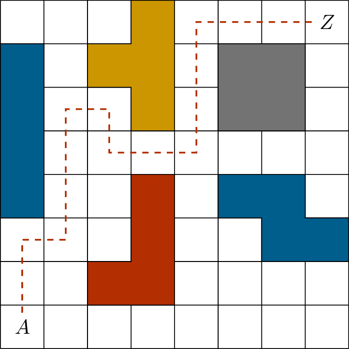
Problem 25.1. In Figure 25.1(a), several Tetris
pieces have been placed on an \(8\times
8\) grid. How many ways are there to get from point \(A\) (the bottom left corner) to point \(Z\) (the top right corner) by a path
through the square in the grid that does not pass through any Tetris
pieces and does not visit a square more than once?
The puzzle, with one sample pathA few useful squares
Count the paths from \(A\)
to \(Z\)!
This is a book, so I can’t ask you to think about the puzzle on your
own for a bit before I reveal the answer. However, I really do think
it’s a good idea for you to think about it: you’ll internalize the ideas
in this chapter better if you come up with some of them on your own
first. You should especially try to think of a way to solve the problem
systematically and with as little brute force as possible: there’s many
paths, so you don’t want to just list them all.
When you’ve done all the thinking you want to do, keep reading.
No rush—take your time.
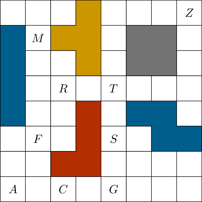
Alright! So: the first insight that cuts down on the work required is
that the square marked \(T\) in
Figure 25.1(b) is special. All paths
from \(A\) to \(Z\) have to go through \(T\) (and they are only allowed to go
through \(T\) once). So every \(A-Z\) path is the union of an \(A-T\) path and a \(T-Z\) path; conversely, the union of every
\(A-T\) path and every \(T-Z\) path is an \(A-Z\) path. This means that to get our
final count, we can multiply the number of paths from \(A\) to \(T\) by the number of paths from \(T\) to \(Z\).
Which graph are all these paths in?
The graph obtained from the \(8\times 8\) grid graph by deleting every
vertex covered by a Tetris piece. Squares like \(A\), \(T\), and \(Z\) are vertices of this graph.
Let’s make up some notation, just for this problem: let \(p(x,y)\) be the number of paths from \(x\) to \(y\). In this notation, we are looking for
\(p(A,Z)\), but we’ve just discovered
that \(p(A,Z) = p(A,T) \cdot
p(T,Z)\).
What is \(p(T,Z)\)?
It is just \(2\): from \(T\), we can go up and then right, or right
and then up, but the grey square Tetris piece stops us from doing
anything else.
Next, we can simplify \(p(A,T)\)
with just a bit of casework. We can arrive at \(T\) either from the left (through the
square marked \(R\)) or from below
(through the square marked \(S\)). So
we can count both kinds of paths separately.
Is it true that \(p(A,T) = p(A,R) + p(A,S)\)?
No: as we’ve defined it, \(p(A,R)\) counts all paths from \(A\) to \(R\), including ones that go through \(T\) first—and we can’t follow those up by
going back to \(T\).
Instead, let’s define a second function \(q(x,y)\), to be the number of paths from
\(x\) to \(y\) that don’t go through \(T\). Now it’s okay to say that \(p(A,T) = q(A,R) + q(A,S)\). Let’s compute
\(q(A,R)\) first, and come back to look
at \(q(A,S)\) second.
Without going through \(T\), every
path from \(A\) to \(R\) must pass through \(F\) first: like our initial identity, this
lets us factor \(q(A,R)\) as \(q(A,F) \cdot q(F,R)\). What’s more, the
paths cannot go through squares \(C\)
or \(M\): if they do, there’s no way to
return! So \(q(A,F)\) can be computed
just by looking at a \(3 \times 2\)
rectangle in the bottom left corner, and \(q(F,R)\) can be computed just by looking at
a \(4 \times 2\) rectangle. I have no
more tricks to suggest here, but there’s not many paths, so we can just
count them: \(q(A,F) = 4\) and \(q(F,R) = 6\).
When we move on to \(q(A,S)\), the
role of certain squares is reversed. The path cannot go through \(F\), because that cuts off our path of
retreat. It must go through \(C\), and
then it must go through \(G\). (There
is only one way to get from \(C\) to
\(G\) at this point.) So we can factor
\(q(A,S)\) as \(q(A,C) \cdot q(G,S)\). Once again, these
are small problems we can solve in just one corner of the grid by
listing out all the paths; you should get \(q(A,C) = 3\) and \(q(G,S) = 8\).
We are now ready to combine the answers we got: \[\begin{aligned}
p(A,Z) &= p(A,T) \cdot p(T,Z) \\
&= \Big( q(A,R) + q(A,S) \Big) \cdot p(T,Z) \\
&= \Big( q(A,F) \cdot q(F,R) + q(A,C) \cdot q(G,S) \Big) \cdot
p(T,Z) \\
&= \Big(4 \cdot 6 + 3 \cdot 8\Big) \cdot 2 = 96.
\end{aligned}\]
Cut vertices
The graph-theoretic concept at work in our solution to Problem 25.1 is the notion of a cut
vertex.
A cut vertex\(x\)
of a graph \(G\) is a vertex such that
\(G-x\) has more connected components
than \(G\). Most commonly, \(G\) is a connected graph, in which case
\(x\) is a cut vertex if and only if
\(G-x\) is not connected.
For example, in the graph representing Problem 25.1, vertex \(T\) is a cut vertex: deleting it separates
\(A\) from \(Z\). (Several other vertices marked in
Figure 25.1(b), such as \(F\) and \(G\), are cut vertices of subgraphs of this
graph.)
The definition of a cut vertex might resemble the definition of a
bridge given in Chapter 9: we defined a
bridge to be an edge that disconnects a graph (or increases the number
of connected components) when we remove it. For this reason, bridges are
sometimes called cut edges.
We know that in a tree, every edge is a
bridge. Which vertices in a tree are cut vertices?
The cut vertices are exactly the vertices
which are not leaves. When a leaf is deleted, a smaller tree is left;
however, deleting a vertex of degree \(k>1\) leaves \(k\) connected components, one for every
neighbor of the deleted vertex.
What are cut vertices good for? It’s hard to give a complete answer
to a question like that in graph theory, because an easy-to-define
concept can pop up in seemingly unrelated questions. On their own, cut
vertices are good in applications because they tell us about the
reliability of computer networks [53] or supply networks [22], just to name two examples. Usually,
identifying the cut vertices does not tell the complete story; in this
part of the textbook, you will learn some more complicated measures of
reliability, as well.
It can also be helpful to know when a graph has a cut vertex no
matter which problem we’re trying to solve, because it can help us break
down the problem into smaller and simpler problems: we saw that in
action in Problem 25.1. Let’s be a bit more
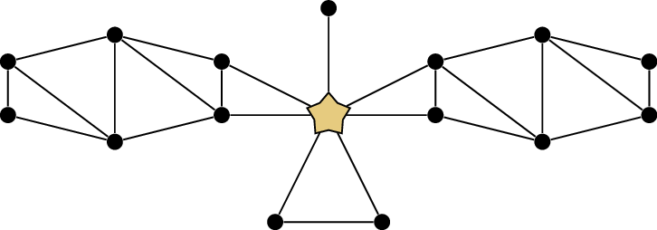
specific about this, though. Given a connected graph \(G\), suppose that \(x\) is a cut vertex of \(G\). Where do we find the subproblems?
Well, we could start by identifying \(G_1,
G_2, \dots, G_k\), the connected components of \(G-x\). But that’s not usually quite what we
want, because none of these connected components “remember” how they fit
together. Instead, we want subgraphs \(H_1,
H_2, \dots, H_k\) that all come together at \(x\). Formally, let \(H_i\) be the subgraph of \(G\) induced by \(V(G_i) \cup \{x\}\); this subgraph includes
only one connected component of \(G-x\), but also keeps track of how that
component is attached to \(x\). An
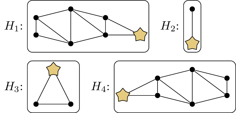
example is shown in Figure 25.2.
A cut vertex in \(G\)\(H_1, H_2, H_3,
H_4\)
Using a cut vertex to break \(G\) down into \(H_1, H_2, \dots, H_k\)
Let’s look at some examples to see how this helps us solve a few of
the problems that have been covered so far in this book.
How does determining whether \(H_1, H_2, \dots, H_k\) are planar help us
decide if \(G\) is planar?
If all \(k\) subgraphs are planar, their plane
embeddings can be combined by placing them around \(x\) like the petals of a rose, so \(G\) is also planar; Figure 25.2 is an example of this.
If one of the subgraphs is not planar, then \(G\) as a whole isn’t planar, either.
How does coloring the graphs \(H_1, H_2, \dots, H_k\) help us find a
coloring of \(G\)?
Though the colorings are not
necessarily compatible “out of the box”, we can permute the colors used
on each subgraph so that all of them give \(x\) the same color. Then, by combining the
colorings, we get a coloring of all of \(G\).
In particular, \(\chi(G) = \max\{\chi(H_1),
\chi(H_2), \dots, \chi(H_k)\}\).
How does finding the largest clique in
\(H_1, H_2, \dots, H_k\) help us find
the largest clique in \(G\)?
A clique in \(G\) must be entirely contained in some
\(H_i\): if we take two vertices other
than \(x\) from different subgraphs,
then they won’t be adjacent.
In particular, \(\omega(G) =
\max\{\omega(H_1), \omega(H_2), \dots, \omega(H_k)\}\).
How does finding a spanning tree of \(H_1, H_2, \dots, H_k\) help us find a
spanning tree of \(G\)?
We can just take the union of the spanning
trees of all the subgraphs. This is always a spanning tree of \(G\), and every spanning tree of \(G\) is obtained in this way, so this can be
used to count the spanning trees of \(G\), or to find a minimum-cost spanning
tree.
There are many more examples, but let’s move on.
2-connected graphs
What happens if we split up a graph at its cut vertices (as in the
previous section) as many times as possible? Eventually, we arrive at a
bunch of smaller graphs with no more cut vertices.
We’ll probably have to use some other tools to solve whatever problem
we were trying to solve in those small graphs. However, maybe the
property of having no cut vertices will make them special somehow? We
should study graphs with no cut vertices to see if we can learn anything
useful about them.
(From the point of view of reliability of a network, graphs with no
cut vertices are also special: they are the graphs that stay connected
even if something happens to one of the vertices.)
I’m going to do something a bit strange with the definition here, and
say that a \(2\)-connected
graph is a connected graph with at least \(3\) vertices and no cut vertices.1 Why is that clause “at least \(3\) vertices” there?
It’s possible to have a \(2\)-vertex
graph with no cut vertices: the graph \(K_2\). (We even saw \(K_2\) among the smaller graphs we got in
Figure 25.2.) However, in many
ways, \(K_2\) is unusual for graphs
with no cut vertices. The reason is that we can rephrase the definition
as saying “For any three different vertices \(x\), \(y\), and \(z\), if \(x\) is deleted, there is still a path from
\(y\) to \(z\).” A graph that doesn’t have three
different vertices satisfies this definition in a trivial way.
Many of the theorems we prove about \(2\)-connected graphs will be false for
\(K_2\), which is why we exclude it
from the definition. This starts with the following theorem, which would
be false if \(K_2\) were considered to
be a \(2\)-connected graph:
Theorem 25.1. A graph \(G\) is \(2\)-connected if and only if any two
vertices of \(G\) lie on a common
cycle. (That is, for all \(x,y \in
V(G)\) there exists a cycle in \(G\) through both \(x\) and \(y\).)
Theorem 25.1 is an if-and-only-if result,
so it is saying two things:
If any two vertices of \(G\) lie
on a common cycle, then \(G\) is \(2\)-connected.
If \(G\) is \(2\)-connected, then any two vertices of
\(G\) lie on a common cycle.
Of these, statement 1 is the easier of the two directions to show, so
we will go ahead and prove it right away; we will return and prove the
second direction of the theorem later in this chapter.
Proof of half of Theorem 25.1. Suppose that any two
vertices of a graph \(G\) lie on a
common cycle. (In particular, \(G\)
must contain at least one cycle, which means that there must be at least
\(3\) vertices.)
Let \(x\) be any vertex of \(G\). To verify that \(G-x\) is connected, let \(y\) and \(z\) be two vertices of \(G-x\). How do we show that in \(G-x\), there is a \(y-z\) path?
Well, in \(G\), there is a cycle
containing both \(y\) and \(z\). We can represent this cycle by a
closed walk \[(x_0, x_1, \dots,
x_{l-1},x_0)\] where \(x_0 = y\)
and \(x_i = z\) for some \(i\). This walk can be split in two: \[(x_0, x_1, \dots, x_{i-1}, x_i) \quad \text{and}
\quad (x_0, x_{l-1}, \dots, x_{i+1}, x_i).\] Both of these walks
represent \(y-z\) paths, and they have
no vertices other than \(y\) and \(z\) in common. Therefore \(x\) (the vertex we delete) can only appear
as a vertex on one of the paths, which means that the other \(y-z\) path survives to \(G-x\). ◻
Through Theorem 25.1, \(2\)-connected graphs have some ties to
topics covered earlier in this book. Here’s a quick example:
Proposition 25.2. If \(G\) is a Hamiltonian graph, then it is
\(2\)-connected.
Proof. If \(G\) has a
Hamilton cycle, then any two vertices of \(G\) lie on that cycle, so \(G\) is \(2\)-connected by Theorem 25.1. ◻
In fact, Proposition 25.2 is a special case of an
earlier result about Hamiltonian graphs. How?
From Corollary 17.3, we know that
all Hamiltonian graphs are tough: if \(k \ge
1\) vertices are deleted, at most \(k\) connected components are left. In the
special case \(k=1\), this tells us
that there cannot be any cut vertices.
Many times in this textbook, we’ve discussed the following kind of
question: if you’ve solved a graph-theoretic problem, how do you give a
short but convincing demonstration that your solution is correct? Let’s
recap a few instances of this:
If two graphs are isomorphic, then we can write down an
isomorphism, and it will be tedious but straightforward to check that it
is an isomorphism.
If two graphs are not isomorphic, a quick way to demonstrate this is
by finding a graph invariant that the two graphs disagree in. However,
finding such an invariant might be hard.
If we want to know the matching number \(\alpha'(G)\) of a bipartite graph, and
we’ve found a large matching \(M\),
that’s only a proof that \(\alpha'(G) \ge
|E(M)|\). What if there’s a larger matching? But by Kőnig’s
theorem (Theorem 14.2), we can always find a vertex
cover \(U\) with \(|E(M)| = |U|\), and use it as a proof that
\(M\) is as large as possible.
If a graph is Hamiltonian, we might still have to work very hard
to find a Hamilton cycle; but once we’ve found it, it is very easy to
check.
What do we do if a graph \(G\) is
not Hamiltonian? Sometimes, if we’re lucky, the graph will not be
tough (as defined in Chapter 17), either. In that case,
after yet more hard work, we can find a set \(S \subseteq V(G)\) such that \(G-S\) has more than \(|S|\) connected components, proving that
\(G\) is not tough and not Hamiltonian.
But there are graphs for which this will not work; we might not always
have a short proof.
If a graph is planar, then we can demonstrate this by drawing a
plane embedding. What if the graph is not planar? Kuratowski’s theorem
(Theorem 22.7) tells us that we
can demonstrate this by finding a subdivision of \(K_{3,3}\) or \(K_5\) inside the graph. Finding the
subdivision might take some work, but checking it takes much less work;
it’s great for busy teachers grading graph theory homework.
These ideas are not just important when applied to individual graphs.
They also often come up when writing a proof! Often, proving that
something does exist is a lot easier than proving that something does
not exist. The ideas here tell us how we can turn the second kind of
proof-writing back into the first kind.
Let’s think about how the idea of short demonstrations applies to
\(2\)-connected graphs.
Suppose a connected graph \(G\) is not \(2\)-connected. How can you demonstrate
this?
You could find a cut vertex \(x\).
Okay, but how do you demonstrate that
\(x\) is a cut vertex?
You’d need to show that \(G-x\) is not connected; Lemma 3.2 can be a
useful tool for this.
It’s less straightforward to consider the other direction: if a graph
is \(2\)-connected, and you want to
prove it, how do you do so? Working directly from the definition, you
could check for every vertex \(x\) that
\(G-x\) is connected, perhaps by giving
a spanning tree of \(G-x\) (but
verifying that a graph is a tree also takes some work). We could also
try to find a collection of cycles so that every pair of vertices lies
on a common cycle in our collection, and apply Theorem 25.1. However, we might need a lot
of cycles to make this happen, and checking them will not be easy.
All this is a lengthy introduction to a new idea: ears, and ear
decompositions.
Let an ear of a graph \(G\) be a path in \(G\) in which every vertex except the first
and last has degree \(2\). From now on,
we will also refer to the vertices of a path except the first and last
as the internal vertices of the path, to make them
easier to refer to.
When we add an ear to a graph \(G\), we pick two different vertices \(x_0\) and \(x_l\) already in \(V(G)\); we add new vertices \(x_1, x_2, \dots, x_{l-1}\) and new edges
\(x_0x_1, x_1x_2, \dots, x_{l-1}x_l\).
This creates the ear represented by the walk \((x_0, x_1, x_2, \dots, x_l)\).
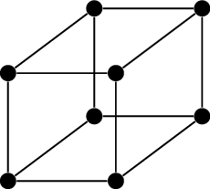
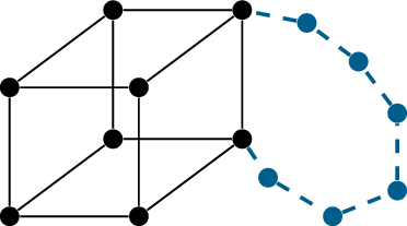
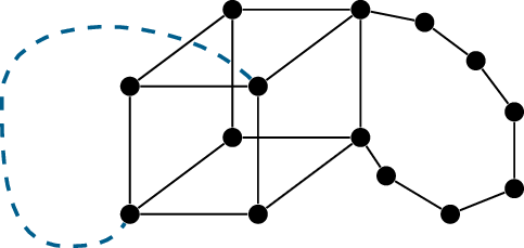
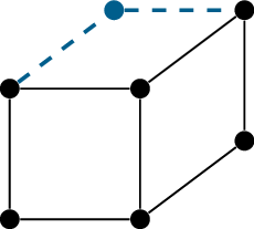
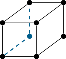
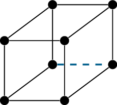
The cube graphThe cube, plus an earThe cube, plus two ears
Adding ears to a cube graph
It’s easier to show what it means to add an ear by means of a
picture, rather than with words. Figure 25.3
shows how, starting with a cube graph (Figure 25.3(a)), we add an ear to arrive
at Figure 25.3(b). This particular ear has
many internal vertices, but that’s not necessary. Adding an edge to a
graph (as in Figure 25.3(c)) is a special case of
adding an ear: it’s adding an ear of length \(1\).
The following lemma is the reason why we introduce ears.
Lemma 25.3. If \(G\) is a \(2\)-connected graph and we add an ear to
\(G\), the resulting graph is also
\(2\)-connected.
Proof. Let \(H\) be a graph
obtained from \(G\) by adding an ear
\(R\): an \(x-y\) path for two different vertices \(x,y \in V(G)\) whose internal vertices only
exist in \(H\). We will prove that the
new graph \(H\) still does not have a
cut vertex.
To do this, we see what happens when we delete a vertex of \(H\):
Suppose we delete a vertex \(z \in
V(G)\) other than \(x\) or \(y\). Because \(G-z\) is connected, all vertices of \(G-z\) are in the same connected component
of \(H-z\). Also, vertices of \(R\) all have a path to \(x\) and \(y\) (because \(R\) is connected), so they are also in that
same connected component: \(H-z\) is
connected.
If we delete \(x\), essentially
the same thing happens. The only change is that an internal vertex of
the ear we added to \(G\) has only only
one path to the connected component of \(G-x\): its path to \(y\) in \(R-x\). Swapping the roles of \(x\) and \(y\), the same thing happens if we delete
\(y\).
If we delete a vertex \(z\)
which is an internal vertex of \(R\),
then \(G\) remains connected, and \(R-z\) is divided into two path components:
one containing \(x\) and one containing
\(y\). Every internal vertex of \(R\) other than \(z\) still has a path to either \(x\) or \(y\), so it is in the same connected
component as the vertices of \(G\).
In all cases, \(H\) remains
connected when we delete a vertex, so it is \(2\)-connected. ◻
In particular, if we start with a cycle and repeatedly add ears, the
result will be connected by Lemma 25.3 and by
induction. We can use this to give a short proof that a graph \(G\) is \(2\)-connected, if we can find a way to
build \(G\) from a cycle inside \(G\) by adding ears. Figure 25.4 shows a way to do
this for the cube graph \(Q_3\).
An ear decomposition of the cube graph
We refer to a demonstration of \(2\)-connectedness via Lemma 25.3 as an ear decomposition. Since
we’d like to use ear decompositions in proofs, let’s give a formal
definition. An ear decomposition of a graph \(G\) is a sequence \(R_1, R_2, \dots, R_k\) of subgraphs of
\(G\) with the following
properties:
\(R_1\) is a cycle.
\(R_i\) is an ear of \(R_1 \cup R_2 \cup \dots \cup R_i\) for all
\(i > 1\).
Each edge of \(G\) is in exactly
one of the subgraphs \(R_i\).
As a consequence, \(G = R_1 \cup R_2 \cup
\dots \cup R_k\).
(The last of these three properties is, as you might remember,
exactly what we mean by a decomposition in general.)
Does such a proof always exist? Yes!
Theorem 25.4. A graph \(G\) is \(2\)-connected if and only if it has an ear
decomposition.
Proof. In both directions of this proof, we will have a
sequence \(R_1, R_2, \dots\) of
subgraphs of \(G\), which we will
either assume to be an ear decomposition or prove to be all or part of
one. To simplify notation, let’s write \(G_i\) for the union \(R_1 \cup R_2 \cup \dots \cup R_i\). In the
case of an ear decomposition, \(R_i\)
should be an ear of \(G_i\), and we
obtain \(G_{i+1}\) from \(G_i\) by adding the ear \(R_{i+1}\).
If \(G\) has an ear decomposition,
then it is \(2\)-connected by repeated
use of Lemma 25.3 in a short induction. Let the
sequence \(R_1, R_2, \dots, R_k\) be
the ear decomposition; then we prove by induction on \(i\) that \(G_i\) is \(2\)-connected. The base case \(i=1\) holds because cycles are \(2\)-connected: deleting any vertex from
\(R_1\) leaves a path. Since \(G_{i+1}\) is obtained from \(G_i\) by adding an ear, Lemma 25.3 is exactly the induction step we
need. Finally, \(G_k = G\), so reaching
\(i=k\) proves that \(G\) is \(2\)-connected.
To prove the other direction of the if-and-only-if statement, we have
to reason in the opposite way from Lemma 25.3,
building up the ear decomposition \(R_1, R_2,
\dots, R_k\) step by step.
We can start by letting \(R_1\) be
any cycle in \(G\). Why does a cycle
exist? Well, we know \(G\) is connected
and has at least three vertices. If \(G\) contained a leaf \(x\), then the only neighbor of \(x\) would be a cut vertex, separating \(x\) from the rest of the graph. This is not
allowed, so \(G\) must have minimum
degree at least \(2\), giving it a
cycle by Theorem 4.4.
It does, but I want to avoid that
argument. We are soon going to use ear decompositions to prove
Theorem 25.1, and I want to make sure that
proof is not circular.
Next, suppose we’ve gotten partway through the process, finding the
subgraphs \(R_1, R_2, \dots, R_i\).
These should satisfy the first two properties of an ear decomposition.
Because we’re not done yet, they don’t have to satisfy the third
property. However, we assume that \(R_1, R_2,
\dots, R_i\) share no edges, and that \(G_i = R_1 \cup R_2 \cup \dots \cup R_i\) is
a subgraph of \(G\). We would like to
make \(G_i\) bigger by adding an ear,
which we’ll call \(R_{i+1}\); however,
we want to add an ear that’s still entirely contained in \(G\).
The first question we ask is this: is \(V(G_i) = V(G)\)? If so, then we’re nearly
done, and continuing the ear decomposition is easy. Pick any edge \(xy \in E(G)\) that is not in \(G_i\), and make that edge (or, more
precisely, the subgraph consisting of \(x\), \(y\), and edge \(xy\)) be the ear \(R_{i+1}\) we add next.
What will steps \(i+2, i+3, \dots\) look like, in this
case?
Since \(V(G_{i+1}) = V(G)\) as well, we’ll stay in
this case until the end. We will add the remaining edges of \(G\), one at a time, as ears of length \(1\).
So it’s the early steps that we have to worry about, when \(V(G_i)\) is still not all of \(V(G)\). In this case, let \(xy\) be any edge where \(x \in V(G_i)\) and \(y \notin V(G_i)\); we will try to construct
an ear that begins with the edge \(xy\).
How do we know such an edge \(xy\) exists?
If there is no such edge, then \(G\) would not have any edges between \(V(G_i)\) and its complement \(V(G) - V(G_i)\), so it would not be
connected.
Since \(G\) is \(2\)-connected, in particular \(G-x\) is connected, so we can find a path
in \(G-x\) from \(y\) to any other vertex. Choose that other
vertex to be a vertex \(z \in V(G_i)\),
not equal to \(x\), of course. There is
a \(y-z\) path in \(G-x\); represent it by a walk \((x_1, x_2, \dots, x_l)\) with \(y = x_1\) and \(z
= x_l\). By setting \(x_0 = x\),
we get an walk \((x_0, x_1, x_2, \dots,
x_l)\); this walk represents an \(x-z\) path that starts and ends in \(G_i\).
Is this path an ear we can add to \(G_i\)?
Not necessarily.
What could be the matter with it?
We don’t know for sure that none of its
internal vertices are in \(V(G_i)\). We
only know this about \(x_1\), because
\(x_1 = y\) was chosen for this
purpose.
To fix this, let \(j>0\) be the
first positive number such that \(x_j \in
V(G_i)\). (Since \(x_l = z\) and
\(z \in V(G_i)\), we know that \(j\) exists, but it’s possible that we
return to \(V(G_i)\) before
reaching \(z\); in that case, \(j<k\).) Now the truncated walk \((x_0, x_1, x_2, \dots, x_j)\) represents an
ear we can add to \(G_i\): if we define
\(R_{i+1}\) to be the path represented
by this walk, then \(R_{i+1}\) is an
ear of \(R_1 \cup R_2 \cup \dots \cup
R_{i+1}\).
How do we know this?
All the internal vertices of \(R_{i+1}\) are not in \(G_i\), so in \(G_i \cup R_{i+1}\), they only have two
neighbors: their neighbors along the path \(R_{i+1}\). This also shows that the edges
\(R_{i+1}\) are not in \(G_i\), because they all involve at least
one of these internal vertices.
To recap, we’ve shown that in all cases, if we’ve picked \(R_1, R_2, \dots, R_i\), then we can
continue by picking \(R_{i+1}\) that
can be part of the ear decomposition. At each step, we add at least one
edge that wasn’t in the partial ear decomposition yet; therefore we’re
guaranteed to eventually build all of \(G\), and obtain an ear decomposition of
\(G\). ◻
An important observation is that no matter how we’ve constructed
\(R_1, R_2, \dots, R_i\), if we haven’t
finished, then we can always choose \(R_{i+1}\) somehow. This makes the algorithm
in the proof a greedy one! The initial cycle \(R_1\) can be any cycle, and later on, each
ear \(R_i\) can be any ear. We don’t
have to worry about making choices that lead us to a dead end later.
In particular, the strategy of picking vertices \(x, y, z\), finding a \(y-z\) path, and seeing where it returns to
\(V(G_i)\) is just one way to guarantee
that we find an ear. We do not have to follow this strategy if have an
alternative. If we’re working with a small graph, such as the cube graph
whose ear decomposition we found in Figure 25.4, then it’s much
easier to just look at the graph and find an ear among the vertices and
edges we haven’t included yet.
Is there a shorter ear decomposition of
the cube graph?
Yes and no. We can work to get to a
spanning subgraph more quickly, at which point we just have edges to
add; for example, we could let \(R_1\)
be a Hamilton cycle in the cube graph. However, we’ll have to add those
edges one at a time, and we’ll still have the same total number of
steps.
In a practice problem at the end of this chapter, I’ll ask you to
prove that this is always true: two ear decompositions of the same graph
always have the same number of pieces.
Induction on ears
Theorem 25.4 can be thought of as an
inductive definition of \(2\)-connected
graphs: a graph \(G\) is \(2\)-connected if and only if it is either a
cycle, or the result of adding an ear to a smaller \(2\)-connected graph. Whenever we have such
a definition of a combinatorial object of any kind, it suggests that
induction is a good strategy for proving properties of such an object.
(See Appendix B for more details about
such definitions.)
Let me begin by giving you an example, which is an application of
\(2\)-connectedness to planar graphs.
(I will be lighter on the geometric details, because they are not the
focus here. In a more careful approach, using Lemma 21.2 to
confirm that all edges must separate two faces is a key step.)
Proposition 25.5. If a planar graph \(G\) is \(2\)-connected, then in every plane
embedding of \(G\), the boundary of
every face is a single cycle.
What are all the ways in which the
boundary of a face might fail to be a cycle?
It’s possible that a face has multiple
boundary walks. This happens when \(G\)
is not connected, and the face touches multiple components of \(G\).
It’s possible that a boundary walk does not represent a cycle because
repeats an edge; we know that this happens when the edge is a
bridge.
Finally, a boundary walk might not repeat any edges, but still repeat
a vertex \(x\). In this case, \(x\) is a cut vertex; intuitively, because
we can draw a closed curve in the face that only crosses the embedding
at \(x\), and separates two parts of
\(G\). In a plane embedding of \(G-x\), the same closed curve will separate
two connected components.
Proof of Proposition 25.5. Since \(G\) is planar, begin by picking a plane
embedding of \(G\).
Since \(G\) is \(2\)-connected, let \(R_1, R_2, \dots, R_k\) be an ear
decomposition of \(G\) (which exists by
Theorem 25.4) and let \(G_i = R_1 \cup R_2 \cup \dots \cup R_i\).
Since \(G_i\) is a subgraph of \(G\), the plane embedding of \(G\) contains a plane embedding of \(G_i\): just erase every vertex and edge of
\(G\) that’s not in \(G_i\).
We will prove by induction on \(i\)
that in this plane embedding of \(G_i\), the boundary of every face is a
single cycle. The base case is \(i=1\).
In this case, \(G_1 = R_1\) is a cycle
; in every plane embedding of the cycle, there are two faces, an inner
face and an outer face, and the entire cycle is the boundary between
them.
Now assume for some \(i>1\) that
in the plane embedding of \(G_{i-1}\),
the boundary of every face is a single cycle. Then \(G_i\) is obtained from \(G_{i-1}\) by adding the ear \(R_i\): a path whose ends are in \(G_{i-1}\), but whose internal vertices are
not. In the plane embedding, this path cannot cross any edges of \(G_{i-1}\), so there must be some face \(F\) in \(G_{i-1}\) that contains it entirely. The
boundary of \(F\) in \(G_{i-1}\) is a cycle, by the induction
hypothesis.
In a plane embedding of the cube graph, each ear divides a
face in two
In \(G_i\), \(F\) is divided by \(R_i\) into two faces \(F_1 \cup F_2\). Their boundaries must share
the path \(R_i\), and divide up the
original boundary of \(F\) somehow. The
only way to do this is by two cycles, each of which follows the boundary
of \(F\) from one endpoint of \(R_i\) to the other, and returns along \(R_i\). See Figure 25.5 for an
illustration of such induction steps in a planar ear decomposition of
the cube graph; in each diagram, the two faces divided by the recently
added ear are shaded.
This completes the induction. Now, Proposition 25.5 follows from the \(i=k\) case, because \(G_k\) is all of \(G\). ◻
In general, inducting on ear decompositions follows the pattern of
this proof. First, we choose an ear decomposition, and verify that the
claim holds for \(R_1\) (a cycle).
Next, we verify that if the claim is true for \(G_{i-1}\), it holds for \(G_i\): in other words, that the claim
continues to hold if we add an ear.
Earlier, we observed that an ear decomposition can be found greedily;
in particular, that we can begin the ear decomposition by choosing \(R_1\) to be any cycle we like. This is
occasionally useful when writing a proof by induction, since we can make
sure that some key vertices end up in \(R_1\).
Of course, if we want to do this, we need to prove that the cycle we
want exists, first. Once we’ve shown Theorem 25.1, it
will be an excellent tool for the base case, because it’s all about
cycles existing. Unfortunately, my plan for Theorem 25.1 is to use an induction on ear
decompositions! So we will need to begin with a silly lemma that will no
longer be necessary once Theorem 25.1 is
there to replace it, but will be useful in that particular proof.
Lemma 25.6. If \(G\) is \(2\)-connected, and \(x\) is any vertex, then \(G\) has a cycle containing \(x\).
Proof. To have any hope of finding a cycle through \(x\), we need to know that \(x\) has two neighbors. Well, if \(x\) had only one neighbor, we’d be able to
delete that neighbor to disconnect \(x\) from the rest of the graph: the
neighbor of \(x\) would be a cut
vertex.
So we can choose two neighbors of \(x\); call them \(u\) and \(v\).
Because \(G\) is \(2\)-connected, \(G-x\) is still connected, and in particular
there is a \(u-v\) path \(P\) in \(G-x\). We obtain a cycle through \(x\) from \(P\) by adding vertex \(x\) and edges \(\{ux,vx\}\) to \(P\). ◻
Theorem 25.1
would be false if we considered \(K_2\)
to be a \(2\)-connected graph, and so
would Lemma 25.6. At which step would the
proof fail, if \(G = K_2\)?
When we talk about a vertex deletion that
would “disconnect \(x\) from the rest
of the graph”, we assume that there is a rest of the graph, which is
false in the case of \(K_2\).
In the next section, we will see two more examples of induction on
ear decompositions, and we will see how Lemma 25.6 fits in.
Finding common cycles
Before we prove Theorem 25.4, we will prove a second
lemma. Unlike Lemma 25.6, this one remains useful
in the study of \(2\)-connected graphs;
it’s not just a tool for this one particular proof.
Lemma 25.7. If \(G\) is \(2\)-connected, and \(u,v,x\) are any three vertices, then \(G\) contains a \(u-v\) path that passes through \(x\).
Proof. By Lemma 25.6, \(G\) contains a cycle containing \(x\). Let \(R_1,
R_2, \dots, R_k\) be an ear decomposition of \(G\) in which \(R_1\) is a cycle containing \(x\), and let \(G_i = R_1 \cup R_2 \cup \dots \cup R_i\).
We will prove by induction on \(i\)
that if \(u\) and \(v\) are any two vertices in \(G_i\), then \(G_i\) contains a \(u-v\) path that passes through \(x\).
When \(k=1\), the graph \(G_1\) consists only of the ear \(R_1\): it is a cycle. No matter where \(u\) and \(v\) are on the cycle, there are two \(u-v\) paths going around the cycle from
\(u\) in either direction, and one of
them passes through \(x\), proving the
base case.
Now assume that for some \(i >
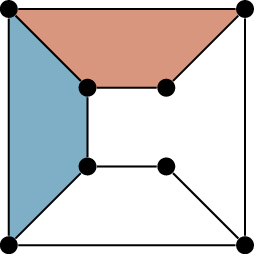
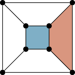
1\) that the paths we want exist in \(G_{i-1}\). Then \(G_i\) is obtained from \(G_{i-1}\) by adding the ear \(R_i\). Let \(u\) and \(v\) be arbitrary vertices of \(G_i\); we consider three cases for where
they might be, illustrated in Figure 25.6.
Case 1. Both \(u\)
and \(v\) are vertices of \(G_{i-1}\). By the induction hypothesis,
\(G_{i-1}\) contains a \(u-v\) path through \(x\). This is also a path in \(G_i\).
Case 2. Only one of \(u\) and \(v\) is a vertex of \(G_{i-1}\); without loss of generality,
\(u \in V(G_{i-1})\) and \(v\) is an internal vertex of \(R_i\). In this case, let \(u'\) be the start or end of \(R_i\). By the induction hypothesis, \(G_{i-1}\) contains a \(u'-v\) path through \(x\). We can extend it to a \(u-v\) path through \(x\) in \(G_i\) if we begin by going from \(u\) to \(u'\) along the ear \(R_i\).
Case 3. Both \(u\)
and \(v\) are internal vertices of
\(R_i\). In this case, let \(u'\) and \(v'\) be the ends of \(R_i\) closer to \(u\) and to \(v\), respectively; that is, \(R_i\) is a path of the form \((u', \dots, u, \dots, v, \dots,
v')\). By the induction hypothesis, \(G_{i-1}\) contains a \(u'-v'\) path through \(x\). We can extend it to a \(u-v\) path through \(x\) in \(G_i\) if we begin by going from \(u\) to \(u'\) and end by going from \(v\) to \(v'\), both along the ear \(R_{i}\).
In all cases, we’ve found the \(u-v\) path through \(x\) we wanted; therefore \(G_i\) contains such a path for any \(u,v \in V(G_i)\). By induction, this is
true for all \(i\) and in particular
for \(i=k\); because \(G_k = G\), this proves the lemma. ◻
With the aid of Lemma 25.3, a
second induction on the ear decomposition is now enough to prove
Theorem 25.1 that any two vertices \(x\) and \(y\) of a \(2\)-connected graph \(G\) lie on a common cycle.
Proof of Theorem 25.1. Let \(x\) and \(y\) be two vertices of a \(2\)-connected graph \(G\); we want to show that there is a cycle
in \(G\) containing both \(x\) and \(y\).
By Lemma 25.6, \(G\) contains a cycle containing \(x\). Let \(R_1,
R_2, \dots, R_k\) be an ear decomposition of \(G\) in which \(R_1\) is a cycle containing \(x\), and let \(G_i = R_1 \cup R_2 \cup \dots \cup R_i\).
We will prove by induction on \(i\)
that if \(y \in V(G_i)\), then \(G_i\) contains a cycle that passes through
both \(x\) and \(y\).
When \(i=1\), this is automatic:
\(G_1 = R_1\) is the cycle we want.
Now assume for some \(i>1\) that
every vertex \(y \in V(G_{i-1})\) lies
on a cycle in \(G_{i-1}\) that also
passes through \(x\). We would like to
prove the same thing for \(G_i\), which
is obtained from \(G_{i-1}\) by adding
the ear \(R_i\). Since we have the
induction hypothesis, we only need to find a cycle through \(x\) and \(y\) when \(y\) is one of the new vertices: an internal
vertex of \(R_i\).
Let \(u\) and \(v\) be the ends of ear \(R_i\). By Lemma 25.6, there is a \(u-v\) path \(P\) in \(G_{i-1}\) passing through \(x\). The paths \(P\) and \(R_i\) have only their ends \(u\) and \(v\) in common: none of the internal
vertices of \(R_i\) are in \(V(G_{i-1})\), and all vertices of \(P\) are. Therefore the union \(P \cup R_i\) is a cycle containing \(x\) (because \(P\) contains \(x\)) and \(y\) (because \(R_i\) contains \(y\)).
By induction, for every \(y \in
V(G_k)\) there is a cycle in \(G_k\) that passes through \(x\) and \(y\); since \(G =
G_k\), this proves the theorem. ◻
Practice problems
Give an example of each of the following:
A \(10\)-vertex graph with \(8\) cut vertices.
A graph with the same number of vertices and edges as in (a), but
only one cut vertex.
A regular graph with only one cut vertex.
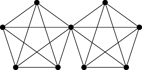
Let \(G\) be a graph consisting
of two copies of \(K_5\) joined at a
vertex:
How many spanning trees does \(G\)
have?
Suppose \(G\) has a cut vertex
\(x\), and that the graphs \(H_1, H_2, \dots, H_k\) are the subgraphs
of \(G\) meeting at \(x\) (as in Figure 25.2).
Explain why knowing the independence numbers \(\alpha(H_1), \alpha(H_2), \dots,
\alpha(H_k)\) is not enough to find \(\alpha(G)\).
Without knowing \(G\), if all I
tell you is the values of \(\alpha(H_1),
\alpha(H_2), \dots, \alpha(H_k)\), what are the minimum and
maximum possible values of \(\alpha(G)\)?
Prove that if \(G\) is \(2\)-connected, and \(H\) is a subdivision of \(G\) (as defined in Chapter 22), then \(H\) is \(2\)-connected.
Find an ear decomposition of:
\(K_{3,3}\).
\(K_{2,5}\).
\(K_{2,n}\) for every \(n\).
You might wonder: is there a shortest ear decomposition in a
graph? In fact, every ear decomposition contains the same number of
pieces.
Suppose that \(G\) has the ear
decomposition \(R_1, R_2, \dots, R_k\),
where \(R_1\) is a cycle of length
\(l_1\) and for each \(i \ge 2\), \(R_i\) is a path of length \(l_i\).
Find the number of edges in \(G\) in
terms of \(l_1, l_2, \dots,
l_k\).
Find the number of vertices in \(G\) in terms of \(l_1, l_2, \dots, l_k\).
If \(G\) has \(n\) vertices, \(m\) edges, and \(k\) ears in an ear decomposition, find a
relationship between \(n\), \(m\), and \(k\) from your answers to the first two
parts.
Conclude that the value of \(k\) is
predetermined by \(G\), and doesn’t
depend on the ear decomposition.
One way to interpret Theorem 25.1 is
that for any two vertices \(x,y\) in a
\(2\)-connected graph \(G\), there are two \(x-y\) paths that share none of their
internal vertices. (Such paths are said to be internally
disjoint, a term we will introduce in Chapter 26.) Here is an
INCORRECT proof of a FALSE generalization:
Claim. If \(G\) is
\(2\)-connected and \(P\) is any \(x-y\) path, there is a second \(x-y\) path \(P'\) that shares no vertices with \(P\) other than \(x\) and \(y\).
“Proof”. Suppose there is no such path \(P'\). That means that all other paths
\(P'\) end up sharing some other
vertex of \(P\). But then, deleting
that vertex of \(P\) destroys all \(x-y\) paths, and so that vertex was a cut
vertex. This cannot happen in a \(2\)-connected graph; contradiction! So a
path \(P'\) must exist.
Point out the mistake in the proof.
Give a counterexample to the claim.
Let \(G\) be a connected graph
with at least \(3\) vertices in which
\(xy\) is a bridge (that is, \(G-xy\) is not connected.)
Prove that either \(x\) or \(y\) is a cut vertex of \(G\). Give an example showing that they’re
not necessarily both cut vertices of \(G\).
Prove that \(xy\) is a cut
vertex of the line graph \(L(G)\).
In a \(3\)-regular graph:
Prove that a vertex \(x\) is a
cut vertex if and only if it is incident to a bridge.
Prove that every cut vertex is incident to either \(1\) or \(3\) bridges.
Prove that the number of cut vertices is even.
The ear decompositions in this chapter are sometimes called
proper ear decompositions. There is also a corresponding notion of
improper ear decompositions. In the improper case, an ear of a graph
\(G\) is also allowed2 to
be a cycle in which every vertex except one has degree \(2\). (That is, when we add an ear, we are
allowed to start and end at the same vertex.)
Prove by example that a graph with an improper ear decomposition
is not necessarily \(2\)-connected.
Instead, improper ear decompositions correspond to
2-edge-connected graphs: connected graphs with no bridges.
(These are a special case of a definition we will make in Chapter 26.)
Prove that if a graph \(G\) has
an improper ear decomposition, then it is 2-edge-connected.
Prove that if a graph is 2-edge-connected, then it has an
improper ear decomposition.
There is an alternate proof of Theorem 25.1 which does not use ear
decompositions. Instead, we prove that any two vertices \(x,y\) lie on a common cycle (equivalently,
there are two \(x-y\) paths with no
internal vertices in common) by inducting on the distance \(d(x,y)\).
For the base case, prove (without relying on any of our other
results) that if \(G\) is \(2\)-connected, then for any edge \(xy \in E(G)\), there is a cycle containing
\(xy\).
For the induction step, we assume that Theorem 25.1 holds for any two vertices at
some distance \(k \ge 1\), and let
\(x\) and \(y\) be two vertices with \(d(x,y)=k+1\). To apply the induction
hypothesis, we let \(z\) be the first
vertex on a shortest \(x-y\) path, so
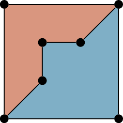
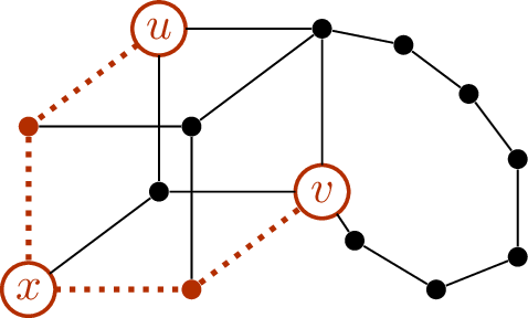
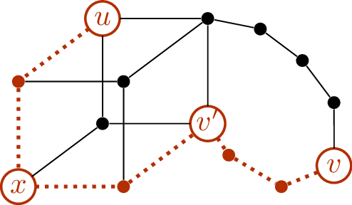
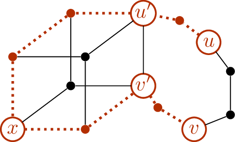
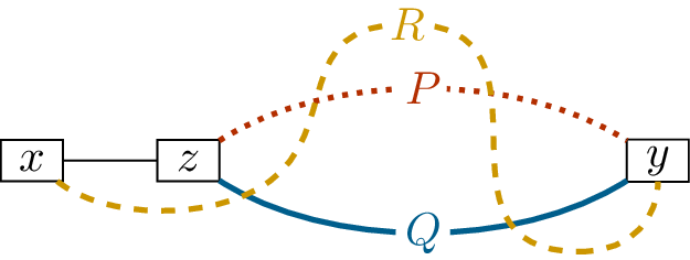
that \(d(z,y)=k\). Let \(P\) and \(Q\) be two internally disjoint \(z-y\) paths, and let \(R\) be an \(x-y\) path in \(G-z\), as shown below:
Prove that no matter how \(R\)
intersects \(P\) and \(Q\), we can find two \(x-y\) paths with no internal vertices in
common.
Footnotes
I am also making this an italicized, “minor” definition,
because in Chapter 26, we will define
what it means for a graph to be \(k\)-connected, and will not need to
refer to this special case again.↩︎
An “improper” ear decomposition should maybe be called a
“not-necessarily-proper” ear decomposition: it could be proper, it just
doesn’t have to be.↩︎