Kőnig’s theorem

The purpose of this chapter

This chapter presents the algorithmic view of matchings in bipartite graphs. The augmenting path algorithm is the most serious algorithm seen in this textbook so far; accordingly, I’ve given it the most serious treatment, with a detailed proof that the algorithm works correctly, and an example of how the algorithm is used. I do not intend to treat every algorithm similarly; this is not a computer science textbook. This is, however, an introductory graph theory textbook, so I hope that this chapter introduces you to the algorithmic side of graph theory.

In my opinion, Kőnig’s theorem (Theorem 14.2) is the right setting to consider the algorithmic questions, because it is a result comparing two optimization problems, which is how we usually encounter matchings in algorithmic applications. Of course, Kőnig’s theorem has its uses in pure mathematics, and Hall’s theorem (Theorem 15.1 in the next chapter) can also be proved by giving an algorithm. However, most uses of Hall’s theorem are about abstractly proving the existence of a perfect matching in a general, incompletely specified family of graphs—and that is the sort of problem we will consider in the next chapter.

Kőnig’s theorem will also become important in Chapter 25 through Chapter 28. We will use it to prove Menger’s theorem (Theorem 27.1). In the other direction, algorithms for the maximum flow problem can be used to solve the bipartite matching problem.

Kőnig’s theorem

As we’ve already seen in Chapter 4 with the notation for minimum degree (\(\delta(G)\)) and maximum degree (\(\Delta(G)\)), graph theorists like to use Greek letters for numerical invariants of graphs. We have recently learned two new such invariants, so let’s learn the notation for them.

Unfortunately, the letters \(\alpha\) (“alpha”) and \(\beta\) (“beta”) here have no particular meaning to help you remember them. There is a meaning to the apostrophe present in \(\alpha'(G)\) but not in \(\beta(G)\): it indicates that the invariant is an “edge version” of another invariant. This means that you can already begin to guess what \(\alpha(G)\) (the “vertex version” of the matching number) might mean: later on, in Chapter 18, you will learn if your guess was right.

Using the new notation, we can rewrite Proposition 13.4, which we stated as an inequality between \(|E(M)|\) (the number of edges in a matching \(M\)) and \(|U|\) (the number of vertices in a vertex cover \(U\)). The new version reads:

Actually, it might not be immediately obvious that Proposition 13.4 and Proposition 14.1 are the same: the first is talking about an arbitrary matching and vertex cover, and the second is only talking about maximum matchings and minimum vertex covers.

However, if Proposition 13.4 holds for all \(M\) and \(U\), then in particular it holds when \(M\) is a maximum matching and \(U\) is a minimum vertex cover, which proves Proposition 14.1. Conversely, if Proposition 14.1 holds, then for any matching \(M\) and vertex cover \(U\), we have \(|E(M)| \le \alpha'(G) \le \beta(G) \le |U|\), proving Proposition 13.4. (The inequalities \(|E(M)| \le \alpha'(G)\) and \(\beta(G) \le |U|\) come from the meanings of the words “maximum” and “minimum”.)

The main theorem of this chapter was proved in 1931 by Dénes Kőnig [63]. Actually, it is ambiguous which result you mean if you say “Kőnig’s theorem”, because Kőnig proved many results in graph theory: he was, in fact, the author of the first graph theory textbook [64], written in 1936.¹ In this textbook, the theorem we’ll call Kőnig’s theorem is the following:

We will prove this theorem by finding an algorithm. Given a matching \(M\), the algorithm will either construct a larger matching \(M'\), or find a vertex cover \(U\) with \(|E(M)| = |U|\).

If we find such a \(U\), what can we conclude?

Since every matching has at most \(|U|\) edges, and \(M\) has exactly \(|U|\) edges, we know that \(M\) is a maximum matching by Proposition 13.4. By similar reasoning, \(U\) is a minimum vertex cover.

However, we know that we cannot always improve a sub-optimal matching simply by adding edges. So what does it take to improve a sub-optimal matching?

Augmenting paths

We will need a set-theoretic operation that is not as well-known as union and intersection, but is the natural operation to consider when tracking changes. (This remains true whether we’re tracking changes made to a matching in a graph, or tracking changes made to a Wikipedia entry, for example.) At its most basic, it’s defined on sets: if \(A\) and \(B\) are two sets, then their symmetric difference \(A \oplus B\) is the set \((A \cup B) - (A \cap B)\): the set containing all elements in \(A\), or in \(B\), but not in both \(A\) and \(B\).

We can think of \(A \oplus B\) as a summary of the changes that need to be made to \(A\) to get \(B\). If we start with \(A\), and “toggle” all the elements of \(A \oplus B\) (removing them from \(A\) if they are in \(A\), and adding them to \(A\) if not), then the result is \(B\).

If we know \(A\) and \(A \oplus B\), what operation on them lets us find \(B\)?

It’s the symmetric difference again: \(B\) is \(A \oplus(A \oplus B)\). The elements in \(A \oplus B\) but not \(A\) are the elements only in \(B\), which we need to add to \(A\); the elements in both \(A\) and \(A \oplus B\) are exactly the ones not in \(B\), which we need to remove.

Which elements does a triple symmetric difference \((A \oplus B) \oplus C\) contain?

The elements contained in an odd number (one, or all three) of the sets \(A, B, C\). This rule generalizes, and can also be used to prove that \(\oplus\) is associative: \((A \oplus B) \oplus C = A \oplus(B \oplus C)\), because the rule applies to both sides.

For example, Figure 14.1 shows a table listing the top ten countries in the International Mathematical Olympiad in 2024 and in 2025. If we think of these lists as sets, we can take the symmetric difference, shown in the third column. This symmetric difference shows the six countries whose status changed from 2024 to 2025: Belarus, the United Kingdom, and Hungary left the top ten list, while Japan, Israel, and Vietnam entered it.

IMO 2024	IMO 2025	2024 ⊕ 2025
United States of America	People’s Republic of China	Belarus
People’s Republic of China	United States of America	United Kingdom
Republic of Korea	Republic of Korea	Hungary
India	Japan	Japan
Belarus	Poland	Israel
Singapore	Israel	Vietnam
United Kingdom	India
Hungary	Singapore
Poland	Vietnam
Türkiye	Türkiye

Rather than continue thinking about competition performance, let’s switch to thinking about graphs. Given two graphs \(G\) and \(H\), the symmetric difference \(G \oplus H\) is the graph with vertex set \(V(G \oplus H) = V(G) \cup V(H)\) and edge set \(E(G \oplus H) = E(G) \oplus E(H)\). We’re taking the symmetric difference of the edge sets, which are the star of the show; we take the union of the vertex sets to be sure that we’ve included the endpoints of every edge we need.

We want to use this idea to see what changes need to be made to get from one matching to another. We are looking for small, incremental changes. So we will compare two matchings \(M\) and \(N\) such that \(M\) only has one more edge than \(N\).

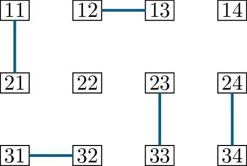
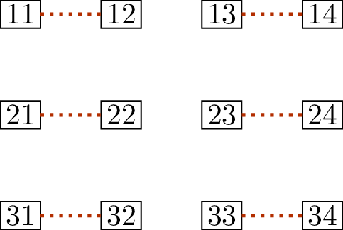
Figure 14.2 shows one such example. To make the drawing more clear, I have not included the edges of the original graph (which you may assume to be a \(3 \times 4\) grid graph). Matching \(M\) (in Figure 14.2(a)) has only \(5\) edges, while \(N\) (in Figure 14.2(b)) is a perfect matching with \(6\) edges.

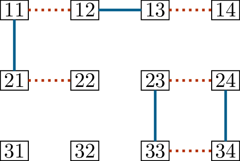
As a graph, \(M \oplus N\) (shown in Figure 14.2(c)) consists of four connected components. Two of them are just isolated vertices, and don’t have a lot to tell us. Another, with the vertices \(\{23,24,33,34\}\), is a cycle, and represents only that the matchings \(M\) and \(N\) match those four vertices in two different ways.

The last component is the most interesting one: the path represented by \((22, 21, 11, 12, 13, 14)\). It’s this component that tells us how to improve matching \(M\): we must swap the two edges \(\{11,21\}\) and \(\{12,13\}\) for the three edges \(\{11, 12\}\), \(\{13,14\}\), and \(\{21,22\}\).

We will call such a subgraph an \(M\)-augmenting path (or just an augmenting path, if it is clear what matching \(M\) it is meant to augment). In general, if \(M\) is a matching in a graph \(G\), then an \(M\)-augmenting path is a path in \(G\) with the following properties:

• The path begins and ends at two vertices that are not covered by \(M\).

• The edges used by the path alternate between edges not in \(M\) and edges in \(M\).

In a symmetric difference of two matchings, we can also see connected components (paths or cycles) that satisfy only the second property, but not the first: we call such paths and cycles \(M\)-alternating.

The length of an \(M\)-augmenting path must be odd, or else it will not end at an uncovered vertex. If it has length \(2k+1\), then the \(1^{\text{st}}, 3^{\text{rd}}, \dots, (2k+1)^{\text{th}}\) edges are not part of \(M\), while the \(2^{\text{nd}}, 4^{\text{th}}, \dots, (2k)^{\text{th}}\) edges are.

If we find a path \(P\) in \(M \oplus N\) that helps us improve \(M\) to be more like \(N\), then we should apply that difference to \(M\) by taking the symmetric difference \(M \oplus P\). This is generalized by the following lemma:

In general, given two matchings \(M\) and \(N\), the symmetric difference \(M \oplus N\) is a graph with maximum degree \(2\): each vertex has at most one incident edge in each matching. The connected components of such a graph are \(M\)-alternating paths and \(M\)-alternating cycles.

Suppose now that, as in our example, \(N\) is a slight improvement over \(M\): \(|E(N)| = |E(M)|+1\). Then, after canceling out the edges common between \(M\) and \(N\), the symmetric difference \(M \oplus N\) still has one more edge from \(N\) than from \(M\). So there must also be at least one connected component of \(M \oplus N\) where this is true!

If a connected component of \(M \oplus N\) is a cycle, can it contain more edges from \(N\) than from \(M\)?

No: to be \(M\)-alternating, exactly half of its edges must be from \(M\), and exactly half must be from \(N\).

If a connected component of \(M \oplus N\) is a path, can it contain more edges from \(N\) than from \(M\)?

Only if it is an \(M\)-alternating path of odd length where the first and last edge both come from \(N\). This is an \(M\)-augmenting path!

In particular, this argument proves that there exists an \(M\)-augmenting path, but not usefully: to find it, we needed to know the bigger matching \(N\). In our proof of Kőnig’s theorem, we will see how to find an \(M\)-augmenting path in a more helpful fashion, but only in bipartite graphs.

The augmenting path algorithm

Let \(G\) be a bipartite graph with bipartition \((A,B)\), and let \(M\) be a matching in \(G\). The main tool we need to prove Kőnig’s theorem is an algorithm for finding an \(M\)-augmenting path.

Our algorithm will be yet another breadth-first search algorithm. However, we will not explore the graph along all possible trajectories, but only along ones that can form an \(M\)-augmenting path.

We are searching for a path between two uncovered vertices, so let’s introduce some notation to help us. Write \(A\) as \(A_0 \cup A_1\), where the vertices in \(A_0\) are uncovered by \(M\) and the vertices in \(A_1\) are covered by \(M\). (That is, \(x \in A_k\) if \(x\) has degree \(k\) in \(M\).) Split \(B\) into \(B_0\) and \(B_1\) in the same way.

Since an augmenting path has odd length, and every path in \(G\) alternates between \(A\) and \(B\), an augmenting path must have one end in \(A_0\) and one end in \(B_0\). We will arbitrarily choose to start our exploration in \(A_0\), with the goal of eventually reaching a vertex in \(B_0\).

To keep track of our progress, let \(A_{\exp}\) and \(B_{\exp}\) be the set of explored vertices in \(A\) and in \(B\), respectively. These will change over the course of the algorithm. Since we start our exploration in \(A_0\), initially \(A_{\exp} = A_0\) and \(B_{\exp} = \varnothing\).

Finally, we will also want to know how we reached the explored vertices: when we add a new vertex \(x\) to \(A_{\exp} \cup B_{\exp}\), we make note of \(f(x)\), the vertex from which we explored \(x\). This will help us find an augmenting path, if one exists.

The augmenting path algorithm repeats the following steps, which I’ve given short names to help us refer to them.

1. Explore: For each vertex \(a \in A_{\exp}\), explore all its neighbors: if a neighbor \(b\) of \(a\) is not already in \(B_{\exp}\), add it, and set \(f(b) = a\). (After the first iteration, this only needs to be done for the vertices newly added to \(B_{\exp}\).)

2. Check: At this step, there are two stopping conditions to check, which conclude the algorithm with different results.

   • Path? If there is a vertex \(b \in B_{\exp} \cap B_0\) (an explored vertex uncovered by \(M\)), stop and return the path represented by the walk \[(b, f(b), f(f(b)), \dots)\] that traces back the vertices from which we reached \(b\), ending at a vertex in \(A_0\). We will show that this is an \(M\)-augmenting path.

   • Cover? If no new vertices were added to \(B_{\exp}\) in the most recent Explore step, stop and return the set \(U\) defined² to be \((A - A_{\exp}) \cup B_{\exp}\). We will show that \(U\) is a vertex cover and \(|U| = |E(M)|\).

3. Match: Otherwise, \(B_{\exp} \subseteq B_1\): all the vertices in \(B_{\exp}\) are covered by \(M\). For each vertex \(b\) added to \(B_{\exp}\) in the most recent Explore step, find the edge \(ab \in E(M)\) incident to \(b\). Explore vertex \(a\) (the vertex that \(b\) is matched to): add it to \(A_{\exp}\), and set \(f(a) = b\).

To prove the correctness of this algorithm, we must show that when the Path or Cover stopping conditions are met, the path really is an \(M\)-augmenting path and the cover really is a vertex cover of the same size as \(M\).

We must also show that the algorithm cannot loop forever. Why must it halt?

At every iteration in which we don’t stop by the Cover condition, we add a new vertex to \(B_{\exp}\), and \(|B_{\exp}|\) is limited in size by \(|B|\).

In practice, this algorithm is applied multiple times. Starting from an initial matching, which does not need to be very good, we repeatedly use the algorithm to grow the matching by one edge. Eventually, we either find a perfect matching, or find a vertex cover that proves we cannot proceed any further. This self-certifying feature, in addition to being theoretically useful in the proof of Kőnig’s theorem, is also practically convenient: it means that we can verify the output of the algorithm independently if we’re not certain that an implementation of it is bug-free.

Which initial matching do we start with? One option is to begin with the empty matching: \(E(M) = \varnothing\).

What does the algorithm do if \(E(M) = \varnothing\)?

We start with all vertices of \(A\) already in \(A_{\exp}\), and all vertices of \(B\) in \(B_0\). If even a single edge exists, we will explore a vertex of \(B_0\) and halt in the first step, returning a path of length \(1\).

When a path of length \(1\) is an \(M\)-augmenting path, what does this mean?

It means that the edge on that path can be added to \(M\) without removing any edges.

Starting from the empty matching, not just the first time we augment the matching but the first few times will typically end equally quickly: they will find an edge between two uncovered vertices. In effect, this is no different from a greedy algorithm. Only once the greedy algorithm would give up, because it cannot add any more edges, does the augmenting path algorithm start finding longer augmenting paths.

Analyzing the algorithm

A common technique when analyzing an algorithm is to prove an invariant of the algorithm. Just like a graph invariant is a property that does not change when the graph is relabeled, an invariant of an algorithm is also a property that does not change—it does not change over the course of the algorithm. Appendix A discusses this proof technique, but this is the first time we really need it in the main body of the textbook.

There are two invariants we track for the augmenting path algorithm: one invariant to help us find an \(M\)-augmenting path, and one invariant that

For the first invariant, we define a path \(P(x)\) for each vertex \(x \in A_{\exp} \cup B_{\exp}\). It is the path represented by \[(x, f(x), f(f(x)), \dots)\] that starts at \(x\) and traces back the vertices from which we reached \(x\), ending at a vertex in \(A_0\). Recall that in the Path stopping condition, this is the path we return, for a vertex \(x \in B_{\exp} \cap B_0\).

Next, we turn our attention to the set \(U = (A - A_{\exp}) \cup B_{\exp}\), which we return if the Cover stopping condition is satisfied. First of all, let’s understand where this set comes from.

If a vertex cover \(U\) satisfies \(|U|=|E(M)|\), can \(U\) ever use both endpoints of an edge in \(M\)?

No: if we select just one endpoint of each edge in \(M\), we’ve already selected \(|E(M)|\) different vertices. Choosing both endpoints of an edge in \(M\) is wasteful and we cannot afford it.

If a vertex cover \(U\) satisfies \(|U|=|E(M)|\), how must it treat \(A_0\) and \(B_0\)?

\(U\) cannot contain any vertices in \(A_0\) and \(B_0\). Again, we’ve already reached \(|E(M)|\) vertices just by selecting a vertex from each edge in \(M\). We can’t select any more without going over our limit, so we can’t select any vertices not covered by \(M\).

These two guiding questions tell us what to do to the vertices we explore. Our initial set \(A_{\exp}\) consists just of \(A_0\): these vertices cannot be part of \(U\). This means that to cover the edges with an endpoint in \(A_0\), we must add all their other endpoints to \(U\). These neighbors are exactly what we put in \(B_{\exp}\) in the Explore step. Next, if a vertex \(b\) we’ve added to \(U\) is an endpoint of an edge \(ab \in E(M)\), we can’t put the other endpoint of \(ab\) in \(U\) as well, so \(a \notin U\). So the vertices matched to \(B_{\exp}\) cannot be part of \(U\), and these are exactly the vertices we put in \(A_{\exp}\) in the Match step.

This logic continues: at each step, vertices we put in \(A_{\exp}\) are vertices we know cannot be part of \(U\), and vertices we put in \(B_{\exp}\) are vertices we know must be part of \(U\). Since we don’t know anything about vertices outside \(A_{\exp} \cup B_{\exp}\) a reasonable first try is to define \(U = (A - A_{\exp}) \cup B_{\exp}\), and we we will see that this turns out to work.

We can define \(U = (A - A_{\exp}) \cup B_{\exp}\) at any point over the course of the algorithm, not just at the end. It is not a vertex cover before the end, but it satisfies an invariant of its own:

Many uses of invariants to study algorithms are proofs by induction in disguise, and you can see that in the proof of Lemma 14.5. Here, we begin with a base case: we show that \(|U| = |E(M)|\) at the beginning of the algorithm. Next, we show that whenever this property holds, it still holds after one more iteration.

Together, Lemma 14.4 and Lemma 14.5 are not enough to draw any conclusions about what happens at the end of the algorithm: we need to see how the stopping conditions contribute.

This completes the proof that the algorithm is correct. It also gives us all the tools we need to prove Kőnig’s theorem.

Using the algorithm

Algorithms like the augmenting path algorithm are not really intended to be performed by hand. Very rarely, if a graph is neither so small that we can find a matching without any algorithms, nor too big to deal with by hand, we can use the algorithm to check a matching we suspect to be optimal. Most of the time, though, you should use a computer. So the purpose of the example here is simply as an illustration, so that you can better understand the algorithm and its proof by seeing it in action. (You will gain even better understanding if you try doing this yourself, and I’ve included a practice problem about this. After you understand the algorithm perfectly, there’s no point.)

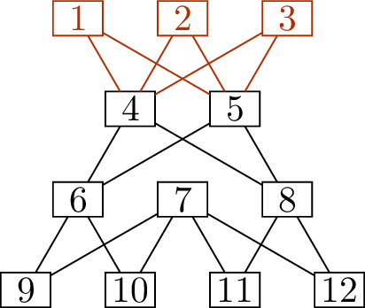
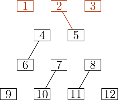
The graph we will use as an example is a graph I’ve called volcano graph, shown in Figure 14.3(a). It does not really have any special properties, but I defined it and named it and I have a hat with the volcano graph on it, so it is my favorite. One of my whims about the definition is that I insist that the top of the volcano graph must always be drawn in red.

Why is the volcano graph bipartite?

All edges have one endpoint in \(\{1,2,3,6,7,8\}\) and one endpoint in \(\{4,5,9,10,11,12\}\).

I have mentioned that the first few rounds of finding augmenting paths are essentially equivalent to a greedy algorithm, so I will skip them to avoid wasting time on cases that don’t help us understand anything. We will begin with the matching \(M\) shown in Figure 14.3(b), with \(E(M) = \{\{2,5\}, \{4,6\}, \{7,10\}, \{8,11\}\}\).

We must make an arbitrary choice between the two sides: let’s say that side \(A\) (the side that we explore from) is \(\{1,2,3,6,7,8\}\). For our initial matching, we start with \(A_0 = \{1,3\}\) and \(B_0 = \{9, 12\}\).

The algorithm proceeds as follows:

1. Explore vertices \(4\) and \(5\), adding them to \(B_{\exp}\), with \(f(4) = 1\) and \(f(5) = 3\).

2. Check the stopping conditions:

   • Is there a Path? No: \(B_{\exp} \cap B_0 = \varnothing\).

   • Is there a Cover? No: we added \(2\) new vertices to \(B_{\exp}\).

3. Match vertex \(4\) to vertex \(6\) and vertex \(5\) to vertex \(2\). Add \(2\) and \(6\) to \(A_{\exp}\), with \(f(2) = 5\) and \(f(6)=4\).

4. Explore vertices \(9\) and \(10\), with \(f(9)=f(10)=6\). As before, add them to \(B_{\exp}\).

5. Check the stopping conditions:

   • Is there a Path? Yes: \(B_{\exp} \cap B_0 = \{9\}\).

   We stop, and output the augmenting path represented by \[(9, f(9), f(f(9)), f(f(f(9))))) = (9, 6, 4, 1).\]

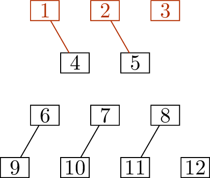
Of the edges on the augmenting path, edge \(\{4,6\}\) is part of \(M\), while edges \(\{1,4\}\) and \(\{6,9\}\) are not. Therefore we improve our matching \(M\) by removing \(\{4,6\}\), adding \(\{1,4\}\) and \(\{6,9\}\) instead. The resulting matching (call it \(M'\)) is shown in Figure 14.4(b).

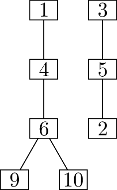
It is common to represent the exploration process by a forest, with the vertices arranged in levels. At the top level are the vertices in \(A_0\); from there, the levels alternate between vertices added to \(B_{\exp}\) in an Explore step and vertices added to \(A_{\exp}\) in a Match step. The forest we get in this example is shown in Figure 14.4(a).

How can we tell which edges of this forest are edges of \(M\)?

They are the edges whose top vertex is in a \(B_{\exp}\) level and whose bottom vertex is in an \(A_{\exp}\) level. In Figure 14.4(a), these are just the edges down from \(\{4,5\}\), but if we had kept going, any edges down from \(\{9,10\}\) would also have been in \(M\).

The forest in Figure 14.4(a) looks like it has other augmenting paths, such as the one represented by \((10, 6, 4, 1)\). Could we have used this path instead?

No: this path only looks like an augmenting path because we stopped before the next Match step, but in reality, vertex \(10\) is covered by \(M\). If we had kept going, we would have found a longer augmenting path.

We have improved the matching, but we’re still not done, so we continue with another round of the algorithm. The edges of the new matching are \(\{\{1,4\}, \{2,5\}, \{6,9\}, \{7,10\}, \{8,11\}\}\), so the uncovered vertices are given by \(A_0 = \{3\}\) and \(B_0 = \{12\}\). Now we:

1. Explore vertices \(4\) and \(5\), adding them to \(B_{\exp}\), with \(f(4) = f(5) = 3\).

2. Check the stopping conditions:

   • Is there a Path? No: \(B_{\exp} \cap B_0 = \varnothing\).

   • Is there a Cover? No: we added \(2\) new vertices to \(B_{\exp}\).

3. Match vertex \(4\) to vertex \(1\) and vertex \(5\) to vertex \(2\). Add \(1\) and \(2\) to \(A_{\exp}\), with \(f(1) = 4\) and \(f(2) = 5\).

4. Explore, but fail to find any vertices: vertices \(1\) and \(2\) are only adjacent to vertices \(4\) and \(5\), which are already in \(B_{\exp}\).

5. Check the stopping conditions:

   • Is there a Path? No: \(B_{\exp} \cap B_0 = \varnothing\).

   • Is there a Cover? Yes: we did not add any new vertices to \(B_{\exp}\).

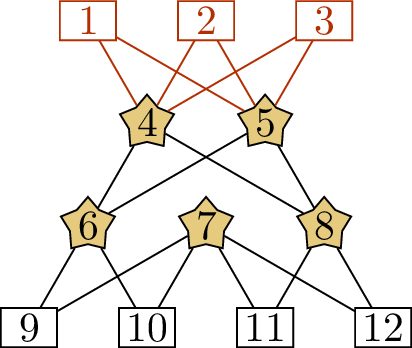
   We stop, and output the vertex cover \[U = (A - A_{\exp}) \cup B_{\exp} = \{6,7,8\} \cup \{4,5\}.\]

Indeed, the vertex \(U = \{4,5,6,7,8\}\) shown in Figure 14.4(c) really is a vertex cover: it consists of the middle two layers of the volcano graph. Every edge between the first two layers is incident to \(4\) or \(5\), every edge between the last two layers is incident to \(6\), \(7\), or \(8\), and every edge between the second and third layer has both endpoints in \(U\). Since \(|U|=|E(M')| = 5\), we conclude that \(M'\) is a maximum matching.

Practice problems

1. Use the augmenting path algorithm to improve the matching in Figure 14.2(a). Does this result in the perfect matching in Figure 14.2(b), or a different one?

2. Viewing the domino tiling in Figure 13.3 as a matching, find a set of \(10\) augmenting paths (with no vertices in common) that will transform it into a perfect matching.

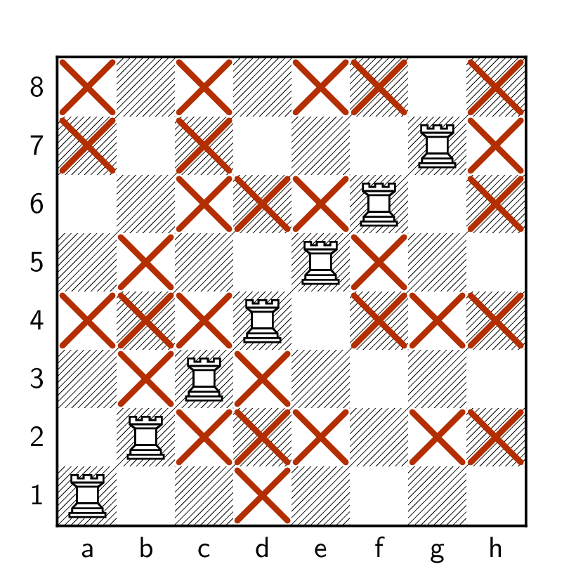
3. On the chessboard below, how many rooks can be placed so that no two rooks occupy the same row or column, and all the crossed-out squares are empty?

   

   A \(7\)-rook solution is shown. Use the augmenting path algorithm to find either an \(8\)-rook solution, or a vertex cover proving that the \(7\)-rook solution is optimal.

4. Let \(G\) be a bipartite graph with bipartition \((A,B)\) and minimum degree \(\delta(G)\); let \(U\) be a vertex cover that does not contain either \(A\) or \(B\).

   1. Prove that \(|U| \ge 2\delta(G)\). When does it follow that \(\alpha'(G) \ge 2 \delta(G)\), and why?

   2. In the case \(|A|=|B|=10\) and \(\delta(G)=3\), give an example of a bipartite graph in which this lower bound is true: \(\alpha'(G) = 6\).

5. If \(G\) is not bipartite, then Proposition 14.1 still guarantees that \(\alpha'(G) \le \beta(G)\), but the two quantities may be different.

   1. Find \(\alpha'(G)\) and \(\beta(G)\) when \(G = C_{2k+1}\), a cycle graph with an odd number of vertices, in terms of \(k\). Verify that they are, in fact, different.

   2. Find a graph \(G\) which satisfies \(\alpha'(G) = \beta(G)\), but is not bipartite.

6. Let \(G\) be a bipartite graph \(G\) with bipartition \((A,B)\) which is \(r\)-regular: every vertex has degree \(r\). Let \(n = |A|\).

   1. Prove that \(|B|=n\) as well, and find \(|E(G)|\) in terms of \(n\) and \(r\).

   2. Prove that a set of \(k\) vertices in \(G\) can cover at most \(kr\) of the edges. What does this say about the size of a vertex cover?

   3. Use Kőnig’s theorem to prove that \(G\) must have a perfect matching.

7. Prove if the augmenting path algorithm is applied to a maximum matching, then \(A_{\exp}\) is the set of all vertices on side \(A\) which are left uncovered by some maximum matching in the graph.

   (You must prove two things: that if \(a \in A_{\exp}\), then there is some maximum matching which does not cover \(a\), and that if \(a \in A - A_{\exp}\), then all maximum matchings cover \(a\).)

Footnotes

1. By a happy coincidence, this is 200 years after Euler first modeled a problem—the problem of the seven bridges of Königsberg—using what we’d now call a graph.↩︎

2. When learning about this algorithm for the first time, this definition may feel like it came out of nowhere! In the next section, we’ll discuss where this formula for the vertex cover comes from.↩︎