Menger’s theorem answers the questions posed at the end of the
previous chapter, and it is the main reason why \(s-t\) connectivity (\(\kappa_G(s,t)\) and \(\kappa'_G(s,t)\) is studied): even if
you want to know how hard it is to disconnect \(s\) from \(t\) for practical purposes, Menger’s
theorem goes a long way toward assuring you that \(s-t\) connectivity is a useful model.
Beyond that, it helps us understand \(\kappa(G)\) (and \(\kappa'(G)\)) as well, often through
Dirac’s fan lemma.
In an introductory course on graph theory, it might be useful to have
a plan for covering just one portion of this chapter, rather than the
whole thing. I can think of two good ways to do this. One option is to
make the proof of Menger’s theorem the final goal of the semester. It is
suitably dramatic, since it is a result that generalizes previous ones
about matchings, answers questions posed in the previous chapter, and is
one of the most difficult proofs in this book, if covered in detail.
Another option is to avoid proving Menger’s theorem, and instead
focus on applications of it. I’ve chosen to include Theorem 27.9 (the Chvátal–Erdős theorem)
as an example of this, for several reasons. It connects the vertex
connectivity \(\kappa(G)\) to two
important topics from earlier chapters: Hamilton cycles and independent
sets. Also, seeing the technique in the proof (illustrated in Figure 27.4) is useful: it shows up over
and over again in the study of Hamilton cycles. If taking this option,
it would still be good to prove Lemma 27.2
if there’s time: the connection between Menger’s theorem and matchings
is also an important application of Menger’s theorem!
Keep in mind that this chapter relies heavily on many different
concepts from previous parts of the book: Kőnig’s theorem from
Chapter 14, Hamilton cycles from
Chapter 17, independent sets from
Chapter 18, and line graphs from
Chapter 20.
Menger’s theorem
We ended the previous chapter with a discussion of optimization
duality, and two instances of it in particular:
The duality between minimizing the number of vertices in an \(s-t\) cut, and maximizing the size of a set
of internally disjoint \(s-t\)
paths.
The duality between minimizing the number of edges in an \(s-t\) edge cut, and maximizing the size of
a set of edge-disjoint \(s-t\)
paths.
We proved in Proposition 26.5 and
Proposition 26.6 that
at the very least, weak duality holds in both pairs: the
largest set of paths is a lower bound on the number of vertices or edges
in the cut.
In 1927, Karl Menger proved [72] that strong duality holds in both
pairs: the largest set of paths is equal to the number of vertices or
edges in the cut.1 We will begin with the vertex
version of Menger’s theorem. I will state it in the following form,
letting Proposition 26.5 (which we’ve
already proved) provide the converse:
Theorem 27.1 (Menger’s theorem). If \(s\) and \(t\) are any two non-adjacent vertices of a
graph \(G\), then \(G\) contains a set of \(\kappa_G(s,t)\) internally disjoint \(s-t\) paths.
The main goal of this chapter is to prove Menger’s theorem.
Many proofs of Menger’s theorem are known, so let me summarize the
origin of the proof presented here. The argument by minimal
counterexample in Lemma 27.3, Lemma 27.4, and Lemma 27.5 is due to Dirac [24]. The remaining cases can
be solved using Kőnig’s theorem (Theorem 14.2),
which is also how the proof is finished in West’s Introduction to
Graph Theory[104].
I prefer to do things this way, because Lemma 27.2 can be used to go in
either direction: it can also let us deduce Kőnig’s theorem from
Menger’s theorem. However, we do not really need the full power of
Kőnig’s theorem; Hall’s theorem would be enough, and in fact Dirac
finished the proof without using any additional results.
The relationship between Menger’s theorem and our earlier results
about matchings extends to algorithms. If we have a complete algorithm
for computing \(\kappa_G(s,t)\), which
finds both an \(s-t\) cut of \(\kappa_G(s,t)\) vertices and a set of \(\kappa_G(s,t)\) internally disjoint \(s-t\) paths, then we can turn it into a
matching algorithm. We do not yet have such an algorithm, and the proof
of Menger’s theorem in this chapter is not suitable for finding one.
However, in Chapter 28, we will look at the
maximum flow problem, which can be used to solve both problems. The
algorithm this gives is more or less the one in Chapter 14, but it’s now a special case of
a more general method.
Kőnig-type graphs
We will begin by understanding \(s-t\) cuts in the special case of what I
will temporarily call “Kőnig-type” graphs. This is not a standard term,
just my name for the case of Menger’s theorem we will address using
Kőnig’s theorem.
We will say that a graph \(G\) with
two vertices designated \(s\) and \(t\) is Kőnig-type if the following
is true:
Vertices \(s\) and \(t\) are not adjacent. (This is a
prerequisite for \(\kappa_G(s,t)\) to
be an interesting problem in the first place: if \(s\) and \(t\) are adjacent, then \(\kappa_G(s,t)=\infty\).)
Every other vertex in the graph is adjacent to \(s\) or to \(t\), but not both.
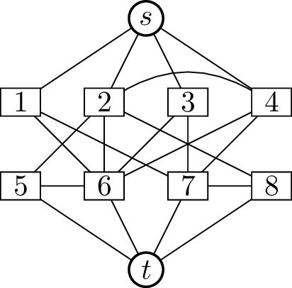
An example of a Kőnig-type graph is given in Figure 27.1(a). Vertices \(1, 2, 3, 4\) are adjacent to \(s\); vertices \(5, 6, 7, 8\) are adjacent to \(t\).
A Kőnig-type graphThe corresponding bipartite graph
The correspondence between Kőnig-type graphs and bipartite
graphsIn Figure 27.1(a),
the sets \(\{1,2,3,4\}\) and \(\{5,6,7,8\}\) are both \(s-t\) cuts. Is there a smaller \(s-t\) cut?
Yes: the \(3\)-vertex set \(\{2, 6, 7\}\) is the unique smallest \(s-t\) cut.
Is there a set of \(3\) internally disjoint \(s-t\) paths to match it?
Yes, represented by the walks \((s,2,5,t)\), \((s,3,6,t)\), and \((s,4,7,t)\).
Given a Kőnig-type graph \(G\), let
\(A\) be the set of vertices adjacent
to \(s\), and let \(B\) be the set of vertices adjacent to
\(t\). We construct a bipartite graph
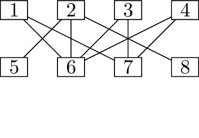
\(H\) from \(G\) by deleting vertices \(s\) and \(t\), as well as all edges not between \(A\) and \(B\). Figure 27.1(b) shows the result of
applying this to the Kőnig-type graph in Figure 27.1(a). (The deletion of vertices
\(s\) and \(t\) is hard to miss, but edges \(24\), \(56\), and \(78\) have also been deleted, which is more
subtle.)
Kőnig’s theorem says that \(\alpha'(H)\), the largest number of
edges in a matching in \(H\), is equal
to \(\beta(H)\), the smallest number of
vertices in a vertex cover of \(H\).
In Figure 27.1(b), can you find a
matching and a vertex cover of equal size?
Edges \(\{16,
25, 37\}\) form a matching, and vertices \(\{2, 6, 7\}\) are a vertex cover of the
same size: every edge is incident to at least one of these three
vertices.
The vertex cover we found is the same set as the \(s-t\) cut in Figure 27.1(a). This is not a
coincidence! Since \(\{2,6,7\}\) is a
vertex cover of \(H\), deleting these
three vertices from \(G\) also
eliminates all edges between \(A\) and
\(B\), which leaves no way to get from
\(s\) to \(t\).
More precisely and more generally, let’s state an equivalence:
Lemma 27.2. Menger’s theorem for a Kőnig-type
graph \(G\) is equivalent to Kőnig’s
theorem for the associated bipartite graph \(H\).
Proof. We’ve already seen a glimpse of the relationship
between \(s-t\) cuts in \(G\) and vertex covers in \(H\), but it will be easier to prove it
formally if we first understand the relationship between internally
disjoint \(s-t\) paths in \(G\) and matchings in \(H\).
A matching \(M\) in \(H\), like the matching with \(E(M) = \{16, 25, 37\}\) we found in
Figure 27.1(b), can always be
turned into a set of internally disjoint \(s-t\) paths of the same size. For each edge
\(xy \in E(M)\), take the path
represented by \((s,x,y,t)\). The
internal vertices of this path are precisely the endpoints of \(xy\), and by the definition of a matching,
two edges in \(M\) share no endpoints.
This means that the paths we get in this way are always internally
disjoint.
Not all \(s-t\) paths are like this;
in Figure 27.1(a), there are very long paths
like the one represented by \((s,2,4,7,3,6,5,t)\). However, each \(s-t\) path must contain an edge \(xy\), where \(x\in A\) and \(y
\in B\), or else it will never reach \(t\). Given a set of internally disjoint
\(s-t\) paths, let \(M\) be the subgraph of \(H\) containing the first edge between \(A\) and \(B\) from each path. Because the paths were
internally disjoint, these edges share no endpoints, so \(M\) is a matching.
This correspondence shows that the largest number of internally
disjoint \(s-t\) paths in \(G\) is equal to the matching number \(\alpha'(H)\). For \(s-t\) cuts in \(G\) and vertex covers in \(H\), the relationship appears to be much
more simple: they are one and the same! But why is this?
In both cases, we are looking for a set of vertices not including
\(s\) or \(t\); a subset \(U
\subseteq V(H)\). The definition of a vertex cover is simpler to
check than the definition of an \(s-t\)
cut: \(U\) is a vertex cover in \(H\) if and only if it contains an endpoint
of every edge \(xy\) with \(x \in A\) and \(y
\in B\). So let’s check that this also describes when \(U\) is an \(s-t\) cut in \(G\).
If \(U\)
is an \(s-t\) cut in \(G\), why must it contain at least one
endpoint of every edge \(xy\) with
\(x\in A\) and \(y \in B\)?
If not, then the walk \((s,x,y,t)\) shows that \(s\) and \(t\) are still in the same connected
component of \(G-U\).
If \(U\)
contains at least one endpoint of every such edge, why is it an \(s-t\) cut in \(G\)?
In this case, \(G-U\) has no edges between \(A\) and \(B\) (or what’s left of them) remaining, so
there is no way to get from \(s\) to
\(t\).
This proves that \(s-t\) cuts in
\(G\) are exactly the same as vertex
covers in \(H\); in particular, \(\kappa'_G(s,t) = \beta(H)\).
We’re now ready to prove the equivalence claimed in the lemma. We
have two pairs of equal quantities, one in \(G\) and one in \(H\):
The largest size of a set of internally disjoint \(s-t\) paths in \(G\) is equal to the matching number \(\alpha'(H)\).
The \(s-t\) connectivity \(\kappa_G(s,t)\) is equal to the vertex
cover number \(\beta(H)\).
Both Menger’s theorem for \(G\) and
Kőnig’s theorem for \(H\) say that the
first pair is also equal to the second pair, so the claims made by the
two theorems are equivalent. ◻
Reducing all other cases
To obtain a proof of Menger’s theorem in general, we must now deal
with graphs which are not Kőnig-type.
We will use a proof by minimal counterexample: a sort of combination
of a proof by induction and a proof by contradiction. Suppose for sake
of contradiction that Menger’s theorem is false for some graphs. Then we
may take \(G\) to be a counterexample
to Menger’s theorem which has as few vertices as possible: a minimal
counterexample.
Sometimes a minimal counterexample is also called a “minimal
criminal”, but I don’t like this terminology, because it’s too much of a
tongue-twister when I try to say it out loud while teaching class. I
don’t mind writing it in a book, though.
What do we do with a minimal counterexample? We try to deduce
additional properties: for example, right now, in the case of Menger’s
theorem, we know that a minimal counterexample is not Kőnig-type,
because then it wouldn’t be a counterexample. The reason minimality is
so important is that very often, we can say, “A minimal counterexample
must have property \(X\), because
otherwise, we could modify it in \(Y\)
way and obtain a smaller counterexample.”
Proofs by minimal counterexample can often be turned into proofs by
induction, but I want to include a proof of this type here, because
they’re a very important exploration technique. When you don’t yet know
whether a theorem is true, proving some properties of a minimal
counterexample is useful in two ways: it is partial progress toward a
proof of the theorem (if it’s true), but it can also help us find a
counterexample (if it’s false).
So let’s see how it works here. The following three lemmas all have
the common hypothesis that a graph \(G\), with designated non-adjacent vertices
\(s\) and \(t\), is a minimal counterexample to
Menger’s theorem. (I will not keep restating these assumptions about
\(G\) each time.) We will prove a few
properties of \(G\), and then put them
together to prove Menger’s theorem. I should warn you that (as in every
book in which the hero has to accomplish three tasks) the third lemma is
the trickiest.
Lemma 27.3. \(G\) cannot contain a vertex \(x\) adjacent to both \(s\) and \(t\).
Proof. Suppose for the sake of contradiction that \(G\) has such a vertex. Then \(x\) must be part of every \(s-t\) cut: if it is not deleted, there is
an \(s-t\) path \(P\) represented by \((s,x,t)\). So every \(s-t\) cut has the form \(U \cup \{x\}\), where \(U\) is an \(s-t\) cut in \(G-x\).
Let \(H = G-x\). Because (as we’ve
just proved) every \(s-t\) cut in \(G\) consists of an \(s-t\) cut in \(H\), plus one extra vertex, we have \(\kappa_G(s,t) = \kappa_H(s,t) + 1\).
But we know that \(H\) is smaller
than the minimal counterexample to Menger’s theorem! So by Menger’s
theorem, \(H\) contains a set of \(\kappa_H(s,t)\) internally disjoint \(s-t\) paths.
All these \(s-t\) paths are also
\(s-t\) paths in \(G\), and we can add one more path to the
set: the path \(P\) defined above.
Therefore \(G\) contains a set of \(\kappa_H(s,t)+1\) internally disjoint \(s-t\) paths. But this is exactly the number
of paths Menger’s theorem promises, so we contradict our assumption that
\(G\) is a counterexample to Menger’s
theorem. ◻
Lemma 27.4. Every vertex in \(G\), other than \(s\) and \(t\), is part of some \(s-t\) cut of size \(\kappa_G(s,t)\).
Proof. Let \(x\) be an
arbitrary vertex of \(G\), and let
\(H = G-x\). As in the previous lemma,
\(H\) is smaller than the minimal
counterexample to Menger’s theorem, so \(H\) contains a set of \(\kappa_H(s,t)\) internally disjoint \(s-t\) paths.
Therefore \(G\) also contains a set
of \(\kappa_H(s,t)\) internally
disjoint \(s-t\) paths. Since \(G\) is a counterexample to Menger’s
theorem, these paths must not be enough: \(\kappa_G(s,t)\) must be bigger than \(\kappa_H(s,t)\). In other words, \(\kappa_G(s,t) \ge \kappa_H(s,t)+1\).
Let \(U\) be an \(s-t\) cut in \(H\) of size \(\kappa_H(s,t)\). Then \(U \cup \{x\}\) is an \(s-t\) cut in \(G\) of size \(\kappa_H(s,t)+1\), because \(G - (U \cup \{x\})\) is exactly the same
graph as \(H - U\). This proves that
\(\kappa_G(s,t) \le \kappa_H(s,t)+1\),
and since we have the reverse inequality already, we know that \(\kappa_G(s,t)\) and \(\kappa_H(s,t)+1\) are equal.
Therefore \(U \cup \{x\}\) is the
\(s-t\) cut containing \(x\) we wanted: it has size \(\kappa_H(s,t)+1 = \kappa_G(s,t)\). ◻
Let \(A\) be the set of all vertices
adjacent to \(s\) in \(G\), and let \(B\) be the set of all vertices adjacent to
\(t\). From Lemma 27.3, we know that \(A\) and \(B\) are disjoint, but we do not (yet) know
if they include every vertex other than \(s\) and \(t\). Both \(A\) and \(B\) are \(s-t\) cuts, though they might have more
than \(\kappa_G(s,t)\) vertices.
Lemma 27.5. \(G\) has no \(s-t\) cuts of size \(\kappa_G(s,t)\) not equal to either \(A\) or \(B\).
Proof. Let \(U\) be an
\(s-t\) cut in \(G\) with \(|U| =
\kappa_G(s,t)\). If \(U\)
contains all of \(A\), then \(U\) must be equal to \(A\), because otherwise \(A\) would be a smaller \(s-t\) cut. Similarly, if \(U\) contains all of \(B\), then \(U\) must be equal to \(B\). So assume, for the sake of
contradiction, that \(U\) does not
contain all of either set: there is some \(x
\in A\) and some \(y \in B\)
such that \(U\) does not contain either
\(x\) or \(y\).
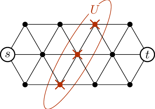
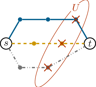
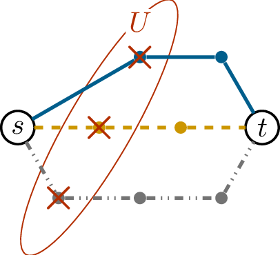
The original graph \(G\)Subproblem 1 (\(L\))Subproblem 2 (\(R\))
The vertices \(x\) and \(y\) will be important eventually, but for
the moment, we simply use \(U\) to
split up the problem of finding internally disjoint \(s-t\) paths in \(G\) into two smaller subproblems. This is
shown by example in Figure 27.2,
which is worth a thousand words. Here are a few words to describe what
we do in general:
Subproblem 1. Take the subgraph of \(G\) induced by \(U\) and all the vertices in the same
connected component of \(G-U\) as \(s\). This does not include \(t\), because in \(G-U\), vertices \(s\) and \(t\) are in different components. But now,
add \(t\) back in, with edges from
every vertex in \(U\) directly to \(t\). Call the resulting graph \(L\) (for “left”, since in our example, it
retains the left half of Figure 27.3).
Subproblem 2. Take the subgraph of \(G\) induced by \(U\) and all the vertices in a different
connected component of \(G-U\) from
\(s\). (This includes \(t\), but not \(s\).) Add \(s\) back in, with edges from \(s\) directly to every vertex in \(U\). Call the resulting graph \(R\) (for “right”).
The vertices \(x\) (in \(A\), but not in \(U\)) and \(y\) (in \(B\), but not in \(U\)) guarantee that the two subproblems are
strictly smaller than \(G\): in \(L\), there is no vertex \(y\), and in \(R\), there is no vertex \(x\). As in Lemma 27.3, the natural next step is to
apply Menger’s theorem to \(L\) and
\(R\). To do this, the first thing we
need to know is \(\kappa_{L}(s,t)\) and
\(\kappa_{R}(s,t)\).
In Figure 27.2,
how do \(\kappa_{L}(s,t)\) and \(\kappa_{R}(s,t)\) compare to \(\kappa_G(s,t)\)?
All three \(s-t\) connectivities are equal.
This is true in general. To find an \(s-t\) cut in \(L\), we must block all ways to get from
\(s\) to \(U\) (since every vertex to \(U\) is adjacent to \(t\)). This also blocks all ways to get from
\(s\) to \(U\) in \(G\) (since before we pass through \(U\), we cannot reach a place where \(G\) and \(L\) disagree), so we get an \(s-t\) cut in \(G\) as well, proving \(\kappa_L(s,t) \ge \kappa_G(s,t)\).
Similarly, \(\kappa_R(s,t) \ge
\kappa_G(s,t)\), because an \(s-t\) cut in \(R\) blocks all ways to get from \(U\) to \(t\), which makes it an \(s-t\) cut in \(G\) as well.
The reverse inequalities \(\kappa_L(s,t)
\le \kappa_G(s,t)\) and \(\kappa_R(s,t)
\le \kappa_G(s,t)\) hold because \(U\) is a cut of size \(\kappa_G(s,t)\) in all three graphs: \(G\), \(L\), and \(R\).
Because \(L\) is strictly smaller
than \(G\), Menger’s theorem holds for
\(L\), giving a set of \(\kappa_G(s,t)\) internally disjoint \(s-t\) paths in \(L\). Since \(|U|
= \kappa_G(s,t)\) and every \(s-t\) path in \(L\) must first pass through \(U\), this set of paths uses each vertex in
\(U\) exactly once. By removing the
last step from each path, we get a set of internally disjoint paths from
\(s\) to every vertex of \(U\).
Because \(R\) is strictly smaller
than \(G\), Menger’s theorem holds for
\(R\), giving a set of \(\kappa_G(s,t)\) internally disjoint \(s-t\) paths in \(R\). Since \(|U|
= \kappa_G(s,t)\) and every \(s-t\) path in \(R\) must first pass through \(U\), this set of paths uses each vertex in
\(U\) exactly once. By removing the
first step from each path, we get a set of internally disjoint paths
from every vertex of \(U\) to \(t\).
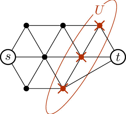
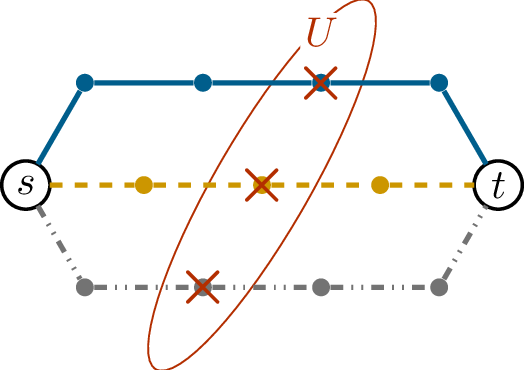
\(s-t\) paths in \(L\)\(s-t\) paths in \(R\)\(s-t\) paths in \(G\)
For each vertex \(u \in U\), the
union of an \(s-u\) path from the first
set and a \(u-t\) path from the second
set is an \(s-t\) path in \(G\). (This is shown for our example in
Figure 27.3.) All \(\kappa_G(s,t)\) paths obtained in this way
are internally disjoint: they cannot intersect in or before \(U\), because that would be an intersection
in \(L\), and they cannot intersect
after \(U\), because that would be an
intersection in \(R\).
But finding a set of \(\kappa_G(s,t)\) internally disjoint \(s-t\) paths in \(G\) contradicts our choice of \(G\): that it was a minimal counterexample
to Menger’s theorem. Therefore the \(s-t\) cut \(U\), which we assumed to exist at the
beginning of this proof, cannot exist in \(G\). ◻
Take a deep breath: Lemma 27.3 was
quick to prove, and Lemma 27.4
was not bad either, but Lemma 27.5 might
have been more than we bargained for. But now, we are ready to finish
the proof of Menger’s theorem in just a few more steps!
Proof of Menger’s theorem (Theorem 27.1).
Suppose for the sake of contradiction that a minimal counterexample to
Menger’s theorem exists: a graph \(G\)
with designated not-adjacent vertices \(s\) and \(t\) which does not have a set of \(\kappa_G(s,t)\) internally disjoint \(s-t\) paths.
By Lemma 27.2 and Kőnig’s theorem, we
know that \(G\) (a counterexample to
Menger’s theorem) cannot be a Kőnig-type graph.
Looking back at the definition of
Kőnig-type graphs earlier in this chapter, what does it mean that \(G\) is not one?
The condition for \(G\) to be Kőnig-type is that every vertex
other than \(s\) or \(t\) is adjacent to \(s\) or \(t\), but not both. So if \(G\) is not Kőnig-type, it must have a
vertex (other than \(s\) or \(t\)) which is either adjacent to both \(s\) and \(t\), or to neither.
Let \(x\) be one such vertex. If
\(x\) is adjacent to both \(s\) and \(t\), this contradicts Lemma 27.3. If \(x\) is adjacent to neither \(s\) nor \(t\), then we need to work harder. First,
apply Lemma 27.4 to find a vertex cut \(U\) of size \(\kappa_G(s,t)\) with \(x \in U\).
Lemma 27.5 says
that in this case, \(U=A\) (the set of
neighbors of \(s\)) or \(U=B\) (the set of neighbors of \(t\)). But neither one is possible, because
\(x \in U\) and \(x\) is not adjacent to \(s\) or \(t\).
In all case, \(G\) contradicts one
of the lemmas we proved, so we conclude that a counterexample to
Menger’s theorem does not exist. ◻
Extensions
Many variants of Menger’s theorem exist. To begin with, a version of
the theorem for \(s-t\) edge cuts also
exists, which is the converse of Proposition 26.6.
Theorem 27.6 (Menger’s theorem, edge version). If
\(s\) and \(t\) are any two vertices of a graph \(G\), then \(G\) contains a set of \(\kappa'_G(s,t)\) edge-disjoint \(s-t\) paths.
It is very tempting (and almost works) to try to prove this version
of Menger’s theorem by applying Theorem 27.1 to the
line graph \(L(G)\).
What is the main problem with trying to
relate \(\kappa'_G(s,t)\) to \(\kappa_{L(G)}(s,t)\)?
The line graph \(L(G)\) doesn’t have vertices called \(s\) and \(t\): its vertices are edges of the original
graph!
To fix the problem, we must modify \(L(G)\) a little.
Proof of Theorem 27.6.
Define a new graph \(H\) in one of the
following two equivalent ways:
Construct \(G'\) from \(G\) by adding two new vertices: one
adjacent only to \(s\) and one adjacent
only to \(t\). Then, let \(H = L(G)\).
Construct \(H\) from \(L(G)\) by adding two new vertices \(s^*\) to \(t^*\). For every vertex of \(L(G)\) which represents an edge incident to
\(s\), make it adjacent to \(s^*\) in \(H\); for every vertex of \(L(G)\) which represents an edge incident to
\(T\), make it adjacent to \(t^*\) in \(H\).
If we construct \(H\) in the first way, what are the two
vertices of \(H\) that correspond to
\(s^*\) and \(t^*\)?
They come from the edges of \(G'\) incident to the two newly-added
vertices.
We must resolve an issue that will otherwise repeatedly bother us
throughout this proof: the relationship between \(s^* - t^*\) paths in \(H\) and \(s-t\) paths in \(G\). In one direction, things work out
nicely. Given a walk \((x_0, x_1, \dots,
x_l)\) in \(G\) where \(x_0 = s\) and \(x_1 = t\), the sequence \((s^*, x_0x_1, x_1x_2, \dots, x_{\ell-1}x_\ell,
t^*)\) is an \(s^* - t^*\) walk
in \(H\), and if the first walk
represents a path, so does the second. (Check this!)
What about the other direction; is it true
that every \(s^* - t^*\) path in \(H\) can be turned into an \(s-t\) path in \(G\) by reversing this process?
No! If it’s been a while since you thought
about paths in \(L(G)\), you should go
back and re-read Chapter 20, but walks in a line graph can do
some things that walks in the original graph cannot: they can contain
segments of the form \((\dots, xy, xz, xw,
\dots)\) with several edges all incident to the same vertex of
\(G\).
However, given an \(s^* - t^*\) path
in \(H\), we can look at the subgraph
of \(G\) containing all the edges that
were internal vertices of the \(s^* -
t^*\) path, and all their endpoints. This is a connected subgraph
of \(G\) containing \(s\) and \(t\), so within it we can find an \(s-t\) path.
By applying Menger’s theorem to \(H\), we get a set of \(\kappa_H(s^*, t^*)\) internally disjoint
\(s^* - t^*\) paths. We know how to
turn each of them into an \(s-t\) path
in \(G\), but we want to know that
we’ll get a set of edge-disjoint paths when we do so.
Suppose \(P\) and \(Q\) are two internally disjoint \(s^* - t^*\) paths in \(H\). When we use them to find two \(s-t\) paths in \(G\), why are those paths
edge-disjoint?
Our first steps with \(P\) and \(Q\) are to go to connected subgraphs of
\(G\) whose edges correspond to
internal vertices of \(P\) and of \(Q\). So even those connected subgraphs have
no edges in common! Therefore the paths we find in them are also
edge-disjoint.
We’ve found a set of \(\kappa_H(s^*,
t^*)\) edge-disjoint \(s-t\)
paths in \(G\), but that’s not enough.
We need \(\kappa'_G(s,t)\)
edge-disjoint \(s-t\) paths, so we must
show that we have at least as many as we need: that \(\kappa_H(s^*, t^*) \ge
\kappa'_G(s,t)\). (The two should be equal, but proving that
is more than we need.)
In other words, we need to show that every \(s^*-t^*\) cut \(U\) in \(H\) is an \(s-t\) edge cut in \(G\). By definition of an \(s^* - t^*\) cut, every \(s^* - t^*\) path in \(H\) passes through some element of \(U\). We’ve already seen that every \(s-t\) path in \(G\) corresponds to an \(s^* - t^*\) path in \(H\): so every \(s-t\) path in \(G\) uses an edge of \(U\). That’s exactly what it means for \(U\) to be an \(s-t\) edge cut!
Therefore applying Menger’s theorem to \(H\) and turning the paths we get back into
paths in \(G\), we get a set of at
least \(\kappa'_G(s,t)\)
edge-disjoint \(s-t\) paths in \(G\), proving the theorem. ◻
Both versions of Menger’s theorem work for multigraphs and for
directed graphs. In the case of multigraphs, Theorem 27.1 is not at all interesting: loops and
parallel edges don’t help us get more internally disjoint paths, and
don’t affect vertex cuts. However, Theorem 27.6 can
be usefully applied to multigraphs: for example, if we have \(17\) parallel edges incident to \(x\) and \(y\), that lets us have \(17\) edge-disjoint paths all taking a step
from \(x\) to \(y\). The proof we gave of Theorem 27.6 works just fine in this
case.
In the case of directed graphs, the notion
of connected components is much less clear, so how should we define
\(s-t\) cuts?
Removing an \(s-t\) cut (either a vertex cut, or an “arc
cut”) from a directed graph should destroy all directed paths from \(s\) to \(t\).
Using Menger’s theorem for directed graphs can be useful for both
vertex and edge cuts, but it takes some work to obtain. In principle,
the proof strategy we used for Menger’s theorem still works for directed
graphs. However, some statements need to be more precise: for example, a
vertex \(x\) should be considered
“adjacent to \(s\)” if there is an arc
from \(s\) to \(x\), but it should be considered “adjacent
to \(t\)” if there is an arc from \(x\) to \(t\). The sets \(A\) and \(B\) are defined accordingly.
How should we modify the construction of
the associated bipartite graph \(H\) of
a Kőnig-type graph \(G\) when \(G\) is a directed graph?
The graph \(H\) should remain undirected; however, it
should only have an edge \(xy\) with
\(x \in A\) and \(y \in B\) if the directed graph \(G\) has an arc from \(x\) to \(y\).
That’s it for the various versions of Menger’s theorem, but there’s a
bit more to be said about its extensions.
First of all, you may feel a bit uncomfortable about the way we’ve
completely forgotten about the global parameters \(\kappa(G)\) and \(\kappa'(G)\), choosing to focus on
\(\kappa_G(s,t)\) and \(\kappa'_G(s,t)\). Well, we can now
return to the global parameters, because for all vertices \(s,t \in V(G)\), we have \(\kappa_G(s,t) \ge \kappa(G)\) and \(\kappa'_G(s,t) \ge \kappa'(G)\).
For instance, we can immediately get the following corollary:
Corollary 27.7. If \(G\) is a \(k\)-connected graph and \(s\) and \(t\) are any two non-adjacent vertices
in \(G\), then \(G\) contains a set of \(k\) internally disjoint \(s-t\) paths.
Given a graph \(G\), a vertex \(s \in V(G)\), and a subset \(T \subseteq V(G)\) with \(s \notin T\), we define an \(s-T\) fan in \(G\) to be a set of paths from \(s\) to vertices in \(T\) that share no vertices except \(s\). (In particular, their ends in \(T\) must be distinct.) To be clear, the
size of an \(s-T\) fan is the number of
paths in the fan.
The notion of \(s-T\) fans was
introduced by Dirac [23].
I suspect that the idea later helped Dirac arrive at the proof of
Menger’s theorem in this chapter, because Lemma 27.5 is all
about combining an \(s-U\) fan and a
\(t-U\) fan to get a set of internally
disjoint \(s-t\) paths. But even before
that, Dirac proved the following lemma as a consequence of Menger’s
theorem.
Lemma 27.8 (Dirac’s fan lemma). If \(G\) is a \(k\)-connected graph, \(T \subseteq V(G)\), and \(s\) is a vertex not in \(T\), then \(G\) contains an \(s-T\) fan of size \(\min\{|T|, k\}\).
Proof. First, let’s deal with the case \(|T| \ge k\), in which case we want to find
an \(s-T\) fan of size \(k\). Define a new graph \(H\) from \(G\) by adding a new vertex \(t\) adjacent to every element of \(T\).
First, we prove that \(\kappa_H(s,t) \ge
k\). Suppose not: suppose that \(U\) is an \(s-t\) cut in \(H\) with \(|U|
\le k-1\). Then \(|U| <
|T|\), so in \(H-U\), there must
be at least some vertices of \(T\)
left, which are in the same connected component as \(T\), and therefore in a different connected
component from \(s\). This means that
in \(G-U\), those vertices of \(T\) are still in a different component from
\(s\), which makes \(U\) a vertex cut in \(G\). But this contradicts our assumption
that \(G\) is \(k\)-connected.
By applying Menger’s theorem to \(H\), we obtain a set of at least \(k\) internally disjoint \(s-t\) paths in \(H\). By removing vertex \(t\) from \(k\) of these paths, what we get is exactly
an \(s-T\) fan in \(G\) of size \(k\).
If \(|T| < k\), then we first
replace \(T\) by a set \(T'\) containing \(T\) of size exactly \(k\). (A \(k\)-connected graph must have at least
\(k+1\) vertices, so this is always
possible.) If we find an \(s-T'\)
fan in \(G\) of size \(k\), then it contains a path from \(s\) to every vertex of \(T'\); in particular, to every vertex of
\(T\). By taking only the paths that go
to \(T\), we get an \(s-T\) fan of size \(|T|\). ◻
By the way, Dirac’s fan lemma is so commonly used that among graph
theorists familiar with it, it is often just called the fan lemma. But I
wanted to disambiguate because I’ve seen this confuse mathematicians
outside this specific subfield of graph theory: there is also a result
in combinatorial topology called the Ky Fan lemma. (Here, Fan is a last
name.)
Cuts and long cycles
Let’s end this chapter by seeing an application of connectivity and
of Dirac’s fan lemma to some topics covered earlier in this book. The
following theorem was proved in 1972 by Václav
Chvátal and Pál Erdős [17], both of whom we’ve met before:
Theorem 27.9. If \(G\) is a graph with at least \(3\) vertices such that the connectivity
\(\kappa(G)\) is at least the
independence number \(\alpha(G)\), then
\(G\) is Hamiltonian.
Proof. If \(\alpha(G)=1\),
then \(G\) can’t be missing even a
single edge between its vertices, in which case it’s definitely
Hamiltonian; so we will assume \(\alpha(G) \ge
2\) and \(\kappa(G) \ge 2\).
It’s a good sign that \(G\) is \(2\)-connected; this means that at least it
has some cycles, by any of the results in Chapter 25. This proof will
proceed by finding longer and longer cycles, until finally getting a
Hamilton cycle.
Let \(C\) be the longest cycle we’ve
found so far. If we’re not done with the proof yet, we assume that it is
not a Hamilton cycle: there is some vertex \(y
\notin V(C)\). Our goal will be to find a longer cycle in \(G\), and to make sure it’s longer, we will
find a cycle that passes through every vertex in \(V(C)\) and also passes through \(y\).
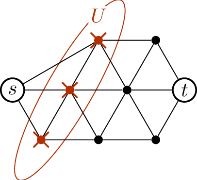
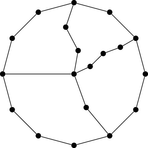
A cycle and a fanVertices \(x_{i+1}\), where
\(i\in I\)A longer cycle is found
Take a \(y-V(C)\) fan in \(G\) with as many paths in it as possible;
by Dirac’s fan lemma, it has size at least \(\min\{|C|, \kappa(G)\}\), but if we’re
lucky, it might be larger. An example is shown in Figure 27.4(a) (with \(y\) in the center). The definition of a fan
does not guarantee that the paths it contains do not share any internal
vertices with \(C\), though I’ve drawn
the fan in this way. However, we can assume that this is true anyway, by
stopping every path in the fan as soon as it reaches a vertex of \(C\).
Let \((x_0, x_1, \dots, x_{l-1},
x_0)\) be a walk representing \(C\). Choosing this walk representation also
gives us a direction to follow along \(C\). If all we have is the cycle, all we
can say is that every vertex on the cycle has two neighbors. With the
walk, we can say that every vertex \(x_i \in
V(C)\) has a vertex \(x_{i+1}\)
that comes after it (taking \(x_l =
x_0\)) and a vertex \(x_{i-1}\)
that comes before it (taking \(x_{-1} =
x_{l-1}\)).
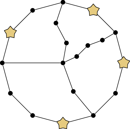
This is important, because I want to define a set of vertices in an
usual way. First, let \(I \subseteq
\{0,1,\dots,l-1\}\) be the set of positions in the cycle where
some path in the \(y-V(C)\) fan ends:
that is, the fan contains a \(y - x_i\)
path whenever \(i \in I\), and not
otherwise. Now, instead of looking at the vertices in the fan, look at
the vertices immediately following them on the path: the set \(\{x_{i+1} : i \in I\}\). These are marked
in Figure 27.4(b).
Looking at this set of vertices appears unmotivated at first, but
it’s a common trick in results about Hamilton cycles, so I want to
explain it a bit. We will soon be trying to find a cycle that mostly
consists of the edges shown in Figure 27.4(a);
although \(G\) has many other edges not
shown in the diagram, we don’t know much about those edges. In this
figure, each vertex \(x_i\) with \(i \in I\) has degree \(3\), so a cycle through them will use two
of their neighbors and neglect the third. Sometimes, \(x_{i-1}\) or \(x_{i+1}\) might be that neglected neighbor,
and so we look at it more closely to find some other edge it might
have!
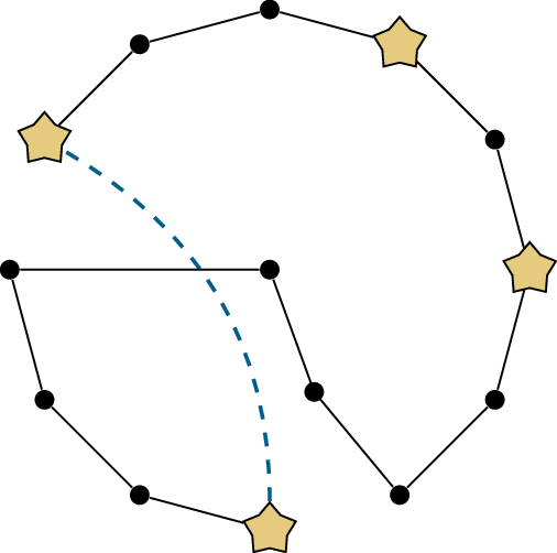
In fact, to get a cycle through \(y\) and every vertex of \(C\), it’s enough to find a single edge
\(x_{i+1} x_{j+1}\) where \(i,j \in I\). An example of such a cycle is
shown in Figure 27.4(c). More formally, the cycle is
obtained as follows:
By deleting edges \(x_i
x_{i+1}\) and \(x_j x_{j+1}\)
from \(C\), we break it into two
pieces: an \(x_{i+1} - x_j\) path \(P\) and an \(x_i
- x_{j+1}\) path \(Q\).
Together, \(V(P) \cup V(Q) =
V(C)\).
By combining the \(y-x_i\) and
\(y-x_j\) paths in the fan, we get an
\(x_i - x_j\) path \(R\) that passes through \(y\) and shares none of its internal
vertices with \(P\) or \(Q\).
The union \(P \cup Q \cup R\)
combines an \(x_{i+1} - x_j\) path, an
\(x_j - x_i\) path, and an \(x_i - x_{j+1}\) path; these paths share no
vertices apart from \(x_i\) and \(x_j\). Therefore \(P \cup Q \cup R\) is an \(x_{i+1} - x_{j+1}\) path. Adding the edge
\(x_{j+1}x_{i+1}\) gives us the cycle
we wanted!
One special case of this might be
confusing: the case where \(j=i+1\), so
that the edge \(x_{i+1}x_{j+1}\) is
actually the edge \(x_{i+1}x_{j+2}\)
which is part of the cycle we started with. What do we do in this
case?
In this case, the path \(R\) we defined is an \(x_i - x_{i+1}\) path passing through \(y\) which is internally disjoint from \(C\), so it can be inserted into the middle
of the cycle between \(x_i\) and \(x_{i+1}\) to get a longer cycle. The same
works if \(i=l-1\) and \(j=0\).
We’ve almost finished the proof, except for one detail: how do we
guarantee that an edge \(x_{i+1}x_{j+1}\) exists? I have to wonder
if Chvátal and Erdős came up with the proof up until now, and only then
asked themselves this question, and that’s how they came up with the
hypotheses of this theorem. After all, we’ve barely used the assumption
about the independence number of \(G\),
so far!
There are two cases. If \(|V(C)| \le
\kappa(G)\), then Dirac’s fan lemma guarantees a fan of size
\(|V(C)|\), which includes a path to
every vertex of \(C\). Therefore every
edge of the cycle is an edge of the type we’re looking for! For example,
the edge \(x_1x_2\) will work, for
\(i=0\) and \(j=1\), because our fan includes an \(y-x_0\) path and a \(y-x_1\) path.
If \(|C| > \kappa(G)\), then
Dirac’s fan lemma only guarantees a fan of size \(\kappa(G)\). At this point, we remember
that \(\kappa(G) \ge \alpha(G)\). If
only we had \(\kappa(G) >
\alpha(G)\), instead! Then we’d know that the set \(\{x_{i+1} : i \in I\}\) cannot be
independent, because it has size \(\kappa(G)\): it’s bigger than the largest
independent set.
But a theorem with \(\kappa(G) >
\alpha(G)\) as a hypothesis would not be the best theorem Chvátal
and Erdős could prove. We can still finish the proof with the hypothesis
\(\kappa(G) \ge \alpha(G)\). For this,
consider the set \(\{x_{i+1} : i \in I\} \cup
\{y\}\), which has at least \(\kappa(G)+1\) vertices, and therefore isn’t
independent. We either get an edge \(x_{i+1}x_{j+1}\) with \(i,j \in I\), which is what we wanted, or an
edge \(x_{i+1}y\) with \(i \in I\), which… isn’t what we wanted.
Can you think of what to do with the edge
\(x_{i+1}y\)?
By combining it with the \(y - x_i\) path in the fan, we get an \(x_i - x_{i+1}\) path through \(y\), internally disjoint to \(C\). This can be inserted into the cycle in
place of going from \(x_i\) to \(x_{i+1}\), obtaining a longer cycle.
To sum it up: we started with an arbitrary cycle which was not a
Hamilton cycle, and were able to make it longer, by incorporating at
least one additional vertex. We can repeat this to grow the new cycle,
too, as many times as necessary. The only way this process can end is by
finding us a Hamilton cycle, proving that \(G\) is Hamiltonian. ◻
You might wonder if the difference between the hypothesis “\(\kappa(G) \ge \alpha(G)\)” in Theorem 27.9, and the hypothesis “\(\kappa(G) > \alpha(G)\)” with which we
could have ended the proof early, is really all that big. Of course, a
theorem with the hypothesis \(\kappa(G) \ge
\alpha(G)\) is better, because it applies to more graphs, but is
it a lot better?
One point in favor of the slightly-better result is that it’s the
best result possible: the theorem could not be improved even further, to
work with the hypothesis \(\kappa(G) \ge
\alpha(G)-1\). One example showing that this is impossible is the
Petersen graph: it is \(3\)-connected
(by a practice problem in Chapter 26) and has
independence number \(4\) (in the usual
diagram with two \(5\)-cycles, an
independent set can contain at most two vertices from each cycle).
However, the Petersen graph is not Hamiltonian (by Proposition 17.1). So
the hypothesis \(\kappa(G) \ge
\alpha(G)-1\) is not always strong enough to guarantee a Hamilton
cycle!
Practice problems
There are \(16\) computers in a
network with the IDs \[10, 12, 13, 14, 20,
21, 23, 24, 30, 31, 32, 34, 40, 41, 42, 43\] consisting of \(2\)-digit numbers with digits \(0\) through \(4\), not both the same. Two computers whose
IDs have the same first digit are directly connected. Additionally, two
computers whose IDs have the same two digits in a different order (such
as \(24\) and \(42\)) have two direct connections between
them, one serving as a backup in case the other fails.
Computers with no direct connection can still communicate by relaying
messages through a sequence of directly connected computers.
You are at computer \(12\) and
your friend is at computer \(34\). How
many intermediate computers, at minimum, need to fail (and stop relaying
messages) before you can no longer communicate with your
friend?
How many connections between computers would need to fail before
you can no longer communicate with your friend?
Justify both answers by an example, as well as a set of paths
demonstrating that the example is the minimum possible.
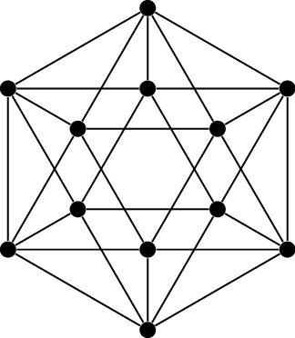
Prove that the skeleton graph of the icosahedron (shown below) is
\(5\)-connected by finding a set of
\(5\) internally disjoint \(s-t\) paths in all three cases: (a) when
\(s\) and \(t\) are adjacent, (b) when the distance
\(d(s,t)\) is \(2\), and (c) when the distance \(d(s,t)\) is \(3\).
Why is the graph not \(6\)-connected?
Prove that the hypothesis of Theorem 27.9 is
the best possible hypothesis for all values of \(\kappa(G)\). That is, for all \(k\ge 1\), find a graph \(G\) with \(\kappa(G) = k\) and \(\alpha(G) = k+1\) which is not
Hamiltonian.
Many of the results about \(2\)-connected graphs in Chapter 25 can now be
obtained much more easily using the results in this chapter.
Prove Theorem 25.1 that any two
vertices in a \(2\)-connected graph lie
on a common cycle, by using Corollary 27.7.
Prove Lemma 25.7 that
for any three vertices \(u,v,x\) in a
\(2\)-connected graph, there is a \(u-v\) path that passes through \(x\), by using Dirac’s fan lemma.
Prove that if \(G\) is \(3\)-connected, then for any three vertices,
\(G\) contains a cycle that passes
through all of them.
More generally, it is true that if \(G\) is \(k\)-connected, then for any \(k\) vertices, \(G\) contains a cycle through all \(k\) of them (in some order); this was the
theorem that Dirac invented his fan lemma to prove. If you’re brave, try
proving this by induction on \(k\).
Footnotes
In the vertex version, we must assume that the vertices
\(s\) and \(t\) are not adjacent, or else there is no
\(s-t\) cut at all. This will be a
recurring assumption for a large part of this chapter.↩︎