Mathematically, the new properties of trees you will learn in this
chapter are nothing special: in Theorem 10.1 and
Theorem 10.2, we will prove how many edges they
have, and later in Lemma 10.5 and
Lemma 10.6, we will learn about their
degree-\(1\) vertices.
All this is notable because it is the point when trees suddenly begin
pulling their weight as theoretical tools that help us solve problems. I
have included two examples of this: the flower garden problem (based on
my experience with recreational math) and Corollary 10.9 (based on my experience with
competition math). In both cases, we are not solving a problem about
trees: we are solving a problem that trees help us solve, because the
problem is somehow related to a connected graph.
Lemma 10.6 is also important because it is what
makes trees such an excellent setting for proofs by induction. (In the
terminology of Appendix B, this lemma gives an
inductive definition of trees.)
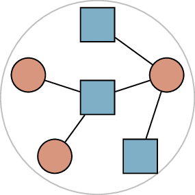
A square garden
Suppose you are designing a garden in the shape of an \(n \times n\) grid. Each square of the grid
can either contain flowers, or be part of a garden path for visitors.
The garden path can bend and fork however you like, but it must be
connected: visitors to the garden must be able to see all of it! Also,
every square with flowers must be next to a square of the garden
path—otherwise, visitors will not be able to see the flowers, and
gardeners will not be able to water them. In both cases, squares that
share only a corner don’t count as being next to each other.
What is the largest number of squares of the grid that can contain
flowers?
\(4 \times 4\)\(5 \times 5\)\(6 \times 6\)
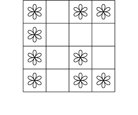
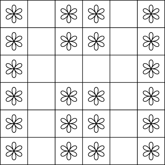
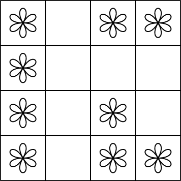
Some high-density flower gardens
I have drawn some solutions for \(4\times
4\), \(5\times 5\), and \(6\times 6\) flower gardens in Figure 10.1, to show you what they can
look like. If you’d like to try it yourself, see if you can manage to
fill \(29\) squares of a \(7\times 7\) garden with flowers.
Solving the problem exactly for large \(n\times n\) grids is, as far as I know,
very difficult even with the help of a computer. However, with the aid
of the material in this chapter, we will able to establish a very good
upper bound on the number of flowers!
To do so, we will need a graph model. First, we must introduce the
grid graph:
Definition 10.1. For any \(m\ge 1\) and \(n\ge 1\), the \(m \times n\) grid graph \(G(m,n)\) is the graph with \(mn\) vertices: points \((x,y)\) where \(x
\in \{1,\dots,m\}\) and \(y \in
\{1,\dots,n\}\). Two vertices are adjacent in \(G(m,n)\) when, viewed as points in the
plane, they are distance \(1\)
apart.
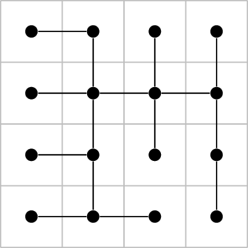
The \(n\times n\) grid graph \(G(n,n)\) represents the \(n\times n\) flower garden: its vertices
correspond to the squares of the grid that forms the garden, and its
edges correspond to adjacent squares. The \(n=4\) case of this is illustrated in
Figure 10.2(a). Of course, \(G(n,n)\) does not tell us anything about
the solution; it is merely the setting where the garden is posed. For
simplicity, we will forget about the grid in favor of the grid graph: we
will say that we plant flowers on some of the vertices of \(G(n,n)\), and put a garden path on the
rest.
We can think of a solution to the flower garden problem as a spanning
subgraph \(H\) of \(G(n,n)\). We include only the edges of
\(G(n,n)\) relevant to checking the
solution. First, keep all edges of \(G(n,n)\) between two vertices that are both
part of of the garden path: these will be necessary to check that the
garden path is connected. Second, for every vertex where a flower is
planted, keep just one edge to an adjacent garden path vertex: these are
necessary to check that the flower is accessible from the garden path.
Figure 10.2(b) and Figure 10.2(c) show how a \(4\times 4\) solution turns into a subgraph
\(H\).
Every valid flower garden turns into a subgraph \(H\), but which subgraphs are the best? They
are the subgraphs with the most degree-\(1\) vertices, because those are the
vertices where flowers are planted. (In principle, a garden path vertex
can also end up having degree \(1\), if
it is an end of the garden path and not necessary to visit any flowers;
however, in that case, we would do better to just plant a flower there,
instead.)
In Chapter 4, we called a vertex with
degree \(1\) a leaf. So we are looking
for a connected spanning subgraph of \(H\) with as many leaf vertices as possible.
Though there is no requirement for \(H\) to be a spanning tree, you may notice
that the graph in Figure 10.2(c) is in fact a tree.
This is no coincidence! Cycles in \(H\)
can only appear in the garden path, but even then, they aren’t
necessary, and we should avoid them: to plant more flowers, we want to
have as little garden path as possible.
How do we maximize the number of leaves in the spanning tree? To do
this, we need to combine some knowledge of vertex degrees with some
facts about the number of edges in a tree, which we will prove later in
this chapter. I will postpone discussing the graph theory behind the
flower garden problem any further until you’ve seen that necessary
background.
Before we move on to more theoretical questions, let me say a bit
about the background of this problem. I made up the flower-garden
formulation of it for this book, but I’ve seen many questions like it
before. Mostly these have not been asked by professional mathematicians,
but by people analyzing board games and video games with a square grid.
However, while writing this chapter, I looked up and found a paper
called “Maximum Leaf Spanning Tree Problem for Grid Graphs” by Li and
Toulouse [69], studying this
exact problem. The paper confirmed that my solutions for the \(4\times 4\) and \(6\times 6\) grid are optimal, and informed
me that solving it is useful for practical questions in the areas of
networking and circuit layout.
Counting edges in trees
By Proposition 9.3 from the previous
chapter, a tree is a connected graph with no cycles. What can we say
about the number of edges this requires?
In Chapter 4, we looked at the
relationship between the number of edges in a graph, and cycles in the
graph. Specifically, Corollary 4.7 tells us that
an \(n\)-vertex graph with at least
\(n\) edges is guaranteed to contain a
cycle.
What does this tell us about the number of
edges in an \(n\)-vertex tree?
To avoid creating any cycles, the tree can
have at most \(n-1\) edges.
If an \(n\)-vertex graph has \(n-1\) edges, must it be a tree?
No: there’s no reason to conclude either
that the graph is connected or that it has no cycles. For example, we
could start with a cycle that has \(n-1\) vertices and edges, then add an
isolated vertex: this is a graph with \(n\) vertices and \(n-1\) edges which is not a tree.
If this were all we knew about trees, then we’d have to stop there,
because \(n\)-vertex graphs without
cycles can have any number of edges between \(0\) and \(n-1\): there’s nothing forcing them to have
any edges. What forces trees to have edges, on the other hand, is the
requirement to be connected: we need some edges to connect the tree!
Let’s explore how many.
Theorem 10.1. A graph with \(n\) vertices and \(m\) edges has at least \(n-m\) connected components.
Proof. We’ll prove this theorem by induction on \(m\): just as in our proof of the handshake
lemma (Lemma 4.1), we will see
what happens as we add edges to a graph one at a time. This time,
however, what we’ll be paying attention to is the number of connected
components.
Our base case is \(m=0\). If a graph
has \(n\) vertices and \(0\) edges, then every vertex is an isolated
vertex, so it is a connected component all by itself. There are always
exactly \(n = n-m\) components.
Now assume that the theorem is true for graphs with \(m-1\) edges, and let \(G\) be a graph with \(n\) vertices and \(m\) edges. Let \(xy\) be an arbitrary edge of \(G\), and consider the \((m-1)\)-edge graph \(G-xy\). By the induction hypothesis, \(G-xy\) has at least \(n-m+1\) connected components.
When we add edge \(xy\), this does
not affect walks from any vertex not in the same connected component as
\(x\) or \(y\). Suppose that a vertex \(z\) has a walk in \(G\) that it did not have in \(G-xy\): a walk of the form \((z, \dots, x, y, \dots)\) or \((z, \dots, y, x, \dots)\). Then if we end
this walk as soon as it first reaches \(x\) or \(y\), we get a \(z-x\) or \(z-y\) walk, so \(z\) must be in the same component as one of
these vertices.
There are two cases for how this can go.
If \(x\) and \(y\) are in the same connected component of
\(G-xy\), then adding edge \(xy\) does not do anything to the components
at all. All the vertices affected are in the same component as \(x\) and \(y\), and so there were already walks
between them in \(G-xy\); they have
nothing to gain. Since \(G-xy\) had at
least \(n-m+1\) components, the same is
true of \(G\).
If \(x\) and \(y\) are in different connected components
of \(G-xy\), then those two components
become the same connected component of \(G\). Any vertex in \(x\)’s component can reach \(y\) (by going to \(x\), then taking edge \(xy\)) and from there, it can reach any
vertex in \(y\)’s component.
Since no other connected components are affected, \(G\) has one component less than \(G-xy\): at least \(n-m\) connected components.
In both cases, \(G\) has at least
\(n-m\) connected components, so the
induction is complete and the statement we want is true for all \(n\) and \(m\). ◻
We can use these ideas to prove a few more characterizations of
trees. Let’s do that, and summarize all our results so far in one big
theorem:
Theorem 10.2. The following conditions for a
graph \(G\) with \(n\) vertices are all equivalent definitions
of a tree:
\(G\) is minimally connected: it is
connected, but deleting any edge will disconnect it.
\(G\) is maximally acyclic: it has no
cycles, but adding any edge will create a cycle.
\(G\) is connected and has no
cycles.
\(G\) is connected and has at most
\(n-1\) edges.
\(G\) has no cycles and at least \(n-1\) edges.
\(G\) is uniquely connected: there is exactly
one path between any two vertices.
Proof. We already know that conditions 1, 2, and 3 are equivalent; we
proved that in the previous chapter.
Let \(G\) be a graph satisfying
these conditions. Then \(G\) has no
cycles, so by the contrapositive of Corollary 4.7, \(G\) has at most \(n-1\) edges. Also, \(G\) is connected, so by Theorem 10.1, it has at least \(n-1\) edges. Now we know that condition 4 and condition 5 are also true.
This doesn’t show that those conditions are equivalent to the first
three. To prove that, we need the reverse implication as well: assuming
only condition 4 or only condition 5, we need to prove one
of the first three conditions.
Suppose that \(G\) satisfies
condition 4. If we delete any
edge from \(G\), we will be left with
at most \(n-2\) edges, so by Theorem 10.1, we will be left with at least \(2\) connected components. Therefore \(G\) is connected, but deleting any edge
will disconnect it: \(G\) satisfies
condition 1.
Suppose instead that \(G\) satisfies
condition 5. If we add any edge
to \(G\), we will get at least \(n\) edges, so by Corollary 4.7, we will get a
cycle. Therefore \(G\) has no cycles,
but adding any edge will create a cycle: \(G\) satisfies condition 2.
This shows that conditions 1–5 are equivalent.
I’ve included condition 6 from a practice
problem at the end of Chapter 9; it’s also
equivalent to the rest, but I won’t prove that here. ◻
In condition 4 of Theorem 10.2, why do we say that \(G\) “has at most \(n-1\) edges”, when in fact we can conclude
\(G\) has exactly \(n-1\) edges?
One of the reasons to have many
characterizations of a tree is to make it as easy as possible to prove
that a graph \(G\) is a tree. So
conditions 4 and 5 are given weaker
statements to make them easier to prove: if \(G\) is connected, and we can easily check
that it cannot have more than \(n-1\)
edges, we don’t need to check that it has exactly that many edges.
From trees to forests
The statement of Theorem 10.1 is an inequality: the number of
connected components is at least \(n-m\). In the case of a tree, \(m = n-1\), and so the number of connected
components is exactly \(n-m\): it is
\(1\). Are there other cases in which a
graph with \(n\) vertices and \(m\) edges has exactly \(n-m\) components?
If \(k\) is the number of connected
components, then the inequality \(k \ge
n-m\) can be rephrased as \(m \ge
n-k\): a graph with \(n\)
vertices and \(k\) connected components
must have at least \(n-k\) edges. To
reach this lower bound, we want to try to use as few edges as possible:
the bare minimum necessary in order to have the \(k\) components we want.
If we want to reach the minimum number of
edges, what should we do in each connected component?
We want each connected component to be a
tree, because this uses the fewest edges to keep the component
connected.
So we define:
Definition 10.2. A forest is a
graph in which every connected component is a tree.
Using condition 3 of Theorem 10.2, we can rephrase this definition;
how?
This condition says that \(F\) is a forest if each connected component
of \(F\) is connected and has no
cycles. Well, of course each connected component is connected. Saying
that each component has no cycles is the same as saying that \(F\) has no cycles at all! Therefore forests
are the same as “acyclic graphs”: graphs with no cycles.
Forests are also exactly the graphs for which the inequality of
Theorem 10.1 becomes an equality. (This statements
includes trees as a special case: in graph theory, a single tree is
still a forest!)
Proposition 10.3. A graph with \(n\) vertices and \(m\) edges has exactly \(n-m\) connected components if and only if
it is a forest.
Proof. Suppose an \(n\)-vertex forest has \(k\) connected components: trees with \(n_1, n_2, \dots, n_k\) vertices, where
\(n_1 + n_2 + \dots + n_k = n\). The
\(i^{\text{th}}\) tree has \(n_i - 1\) edges, so the total number of
edges in the forest is \[(n_1 - 1) + (n_2 -
1) + \dots + (n_k - 1) = (n_1 + n_2 + \dots + n_k) - k = n - k.\]
Since \(m = n-k\), we have \(k = n-m\), proving one direction of the
proposition.
To prove the other direction, let \(G\) be a graph with \(n\) vertices, \(m\) edges, and exactly \(n-m\) connected components, and suppose for
the sake of contradiction that \(G\) is
not a forest: some component of \(G\)
is not a tree. Then \(G\) contains a
cycle; let \(e\) be any edge on this
cycle.
By Lemma 9.2, \(e\) is not a bridge, so \(G-e\) has the same number of connected
components as \(G\): it has \(n-m\) components. But \(G-e\) has \(n\) vertices and \(m-1\), so by Theorem 10.1, \(G-e\) must have at least \(n-m+1\) connected components:
contradiction! So \(G\) must be a
forest. ◻
Leaves in trees
To solve the flower garden problem, we were interested in the number
of leaves (degree \(1\) vertices) of a
spanning tree of the \(n\times n\) grid
graph. Now that we know the number of edges in a tree, the handshake
lemma is sufficient to get a fairly precise upper bound.1
Proposition 10.4. A connected subgraph of the
\(n\times n\) grid graph can have at
most \(\frac23 (n^2+1)\) leaves, and
therefore an \(n\times n\) flower
garden can have at most \(\frac23(n^2+1)\) flowers.
Proof. Let \(H\) be a
connected subgraph of \(G(n,n)\). We
know that \(H\) has \(k\) vertices for some \(k \le n^2\), and by Theorem 10.1, we know that \(H\) has at least \(k-1\) edges.
Suppose that \(H\) has \(l\) leaves. The remaining \(k-l\) vertices of \(H\) can have degree at most \(4\), because the vertices of \(G(n,n)\) have degree at most \(4\). Therefore if we add up the degrees of
all \(k\) vertices of \(H\), we get a total of at most \[\underbrace{1 + 1 + \dots + 1}_{l \text { times}}
+ \underbrace{4 + 4 + \dots + 4}_{k-l \text{ times}} = l + 4(k-l) =
4k-3l.\] By the handshake lemma, this total must be equal to
twice the number of edges in \(H\),
giving us the inequality \[4k - 3l = 2|E(H)|
\ge 2(k-1).\] Solving for \(l\),
we get \(3l \le 2k+2\), or \(l \le \frac23(k+1)\). Since \(k \le n^2\), we obtain the bound we wanted:
\(l \le \frac23(n^2+1)\). ◻
The inequality in Proposition 10.4 is
not quite the best possible: it is impossible to reach exactly \(\frac23(n^2+1)\) flowers. For example, the
garden in Figure 10.1(c) has \(22\) flowers, while \(\frac23(6^2 + 1) = 24 \frac23\). (I have
written the answer as a mixed integer, which is unusual in advanced
math, to make it clear that the bound rounds down to \(24\).)
Part of the gap is due to number theory: actually, \(\frac23(n^2+1)\) is never an integer for
any \(n\), so the sharper bound \(\frac23n^2\) is also true. Part of the gap
is that we can never obtain the ideal scenario where all vertices of
\(H\) have degree \(1\) or \(4\). However, the true answer to the
problem is always very close to \(\frac23
n^2\), as I will ask you to prove in one of the practice problems
at the end of this chapter.
In this application, we wanted to achieve the maximum number of
leaves possible; it is also often useful to know what the minimum number
of leaves is.
Lemma 10.5. Every tree with at least two vertices
has at least two leaves.
Proof. Consider a tree with \(n\) vertices, \(l\) of which are leaves. When \(n\ge 2\), it is impossible for the tree to
contain degree-\(0\) vertices: such a
vertex is an isolated vertex, and cannot be part of a larger connected
graph. Therefore the remaining \(n-l\)
vertices have degree at least \(2\).
We can now apply the handshake lemma, as we did in the proof of
Proposition 10.4. We know that the sum of all
\(n\) degrees in the tree is \(2n-2\): twice the number of edges. However,
we also know that the sum is at least \[\underbrace{1 + 1 + \dots + 1}_{l \text { times}}
+ \underbrace{2 + 2 + \dots + 2}_{n-l \text{ times}} = l + 2(n-l) =
2n-l.\] From the inequality \(2n-l \le
2n-2\), we naturally deduce \(l \ge
2\): the tree must have at least two leaves. ◻
Why is it that we have a \(\le\) inequality (\(2n-l \le 2n-2\)) in this proof, but we had
a \(\ge\) inequality (\(4k-3l \ge 2k-2\)) in the proof of
Proposition 10.4?
In this proof, \(2\) is a lower bound on the degree of the
non-leaf vertices; in the previous proof, \(4\) was an upper bound on the degree of the
non-leaf vertices.
In the proof of Lemma 10.5, I used the sum of degrees to show off this approach a second time, but there is at least one more short proof. Given a tree with at least two vertices, take any longest path \(P\). The endpoints of \(P\) cannot have any neighbors outside \(P\), or else we could make the path even longer. They cannot have more than one neighbor on \(P\), or else a cycle would be formed. Therefore both endpoints of \(P\) have degree \(1\) in the tree: they are the two leaves we were looking for. (We need the tree to have at least two vertices to guarantee that \(P\) has two endpoints of degree \(1\), rather than a single vertex of degree \(0\).)
Leaves in the trees with \(5\) vertices
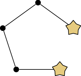
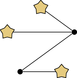
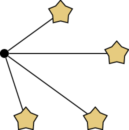
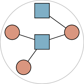
Figure 10.3 shows all three possible
\(5\)-vertex trees, up to isomorphism,
with the leaves marked. You can see that the number of leaves can vary;
in this case, it varies from \(2\) (on
the left) to \(4\) (on the right).
Is it always possible to have an \(n\)-vertex tree with exactly \(2\) leaves?
Yes: the path graph \(P_n\) is a tree, because it is connected
and has \(n-1\) edges, and only the
start and end of the path are leaves.
For an \(n\)-vertex tree, what is the maximum number
of leaves?
It is \(n-1\) (at least when \(n>2\)): imitating the last tree in
Figure 10.3, the graph with a single
central vertex adjacent to \(n-1\)
leaves is an \(n\)-vertex tree.
When \(n>2\), all \(n\) vertices cannot be leaves, because then
the degree sum would be \(n\), which is
less than \(2n-2\). However, this is
achievable when \(n=2\): the only \(2\)-vertex tree, \(P_2\), has \(2\) leaves.
Since the path graph (the tree with as few leaves as possible) has a
name, we should give the tree with as many leaves as possible a name,
too.
Definition 10.3. For all \(n \ge 1\), the star graph\(S_n\) is the tree with \(V(S_n) = \{1,2,\dots,n\}\) and \(E(S_n) = \{12, 13, \dots, 1n\}\).
As with the path graph, not everyone can agree on whether the \(n\)-vertex star graph should be \(S_n\) (because it has \(n\) vertices) or \(S_{n-1}\) (because it has \(n-1\) leaves), but I will go with the first
option for the sake of consistency.
Induction on trees
Why is it important to have leaves? Because when a tree has leaves,
we can pluck them to make the tree a tiny bit smaller.
Lemma 10.6. If \(T\) is a tree and \(x\) is a leaf of \(T\), then \(T-x\) is also a tree.
Proof. We have an abundance of conditions in Theorem 10.2 that we can check to prove this
lemma. I think the easiest one to use is condition 5.
The graph \(T-x\) has no cycles
because it’s a subgraph of \(T\), which
itself has no cycles. If \(T\) has
\(n\) vertices and \(n-1\) edges, then \(T-x\) has \(n-1\) vertices and \(n-2\) edges (because deleting \(x\) also deletes the single edge incident
to \(x\)). The number of edges is one
less than the number of vertices, so condition 5 of Theorem 10.2 is satisfied: \(T-x\) is a tree. ◻
Lemma 10.6 is useful in a proof by induction. In
Appendix B, I explain why it is
important to write your induction proofs backward: having assumed the
induction hypothesis for \((n-1)\)-vertex graphs, we must consider an
\(n\)-vertex graph and remove a vertex
from it to apply the induction hypothesis. Lemma 10.6 gives us a
convenient vertex to remove: if we are proving a theorem by induction
about trees, then we can remove a leaf from an \(n\)-vertex tree to get an \((n-1)\)-vertex tree.
Let me give you a couple examples of such proofs.
Our first example will eventually turn out to be silly: induction is
not needed here. In Chapter 13, we will look at the
property in this example again, and prove a more general result:
Theorem 13.1. With this theorem,
Proposition 10.7 will become a
corollary with a one-line proof. For now, though, it is a good way to
practice induction on trees.2
Proposition 10.7. The vertices of every tree can
be colored red and blue such that no two vertices of the same color are
adjacent.
Proof. We induct on \(n\),
the number of vertices in the tree. When \(n=1\), there is only one vertex, so we may
give it any color we like without violating the condition.
Now assume, for some \(n \ge 2\),
that every \((n-1)\)-vertex tree has a
red-and-blue coloring in which no two vertices of the same color are
adjacent. (Such a red-and-blue coloring is called a \(2\)-coloring, as a special case of a
definition from Chapter 19.) Let \(T\) be an arbitrary \(n\)-vertex tree; we will show that \(T\) also has a \(2\)-coloring.
Let \(x\) be a leaf of \(T\) (which exists by Lemma 10.5), and let \(y\) be its only neighbor in \(T\). By Lemma 10.6, \(T-x\) is also a tree; it has \(n-1\) vertices, so by the induction
hypothesis, it has a \(2\)-coloring.
To color \(T\), first give every
vertex the same color that it had in \(T-x\). Then, color \(x\) by the following rule: if \(y\) is red, color \(x\) blue, and if \(y\) is blue, color \(x\) red. This rule ensures that \(x\) and \(y\) do not have the same color; the same is
true for every other pair of adjacent vertices, because they were
already adjacent in \(T-x\), and \(T-x\) was given a \(2\)-coloring.
This shows that \(T\) also has a
\(2\)-coloring, completing the
induction step. By induction, trees with any number of vertices have
\(2\)-colorings, completing the
proof. ◻
The proof of Proposition 10.7 is not just a proof:
like many proofs by induction, it contains a recursive algorithm. Given
an \(n\)-vertex tree, we can color it
by choosing a leaf, removing it, and applying the coloring algorithm to
the \((n-1)\)-vertex tree that remains,
before putting back the leaf we removed and coloring it as the \(n\)th vertex. Although the
recursive algorithm proceeds backwards from an \(n\)-vertex tree to a \(1\)-vertex tree, if you think about the
order in which vertices are colored, it will appear as though we started
from \(1\) vertex and grew the tree by
adding a succession of leaves, coloring them as we go. Figure 10.4 shows an example of
coloring a \(6\)-vertex tree using this
strategy.
Can you use the proof to deduce how many
\(2\)-colorings a tree has?
In the induction step of the proof, the
color of \(x\) was forced: it had to be
the opposite color of \(y\). Similarly,
at every previous step, the color of the leaf is forced. However, in the
base case, we could give the single vertex of a \(1\)-vertex tree either color. So there are
two \(2\)-colorings possible, based on
which color we chose at that step. (They are opposites of each other:
one is obtained from the other by switching red and blue.)
In most proofs by induction, the full power of Lemma 10.5 is not necessary: a single leaf is
enough. Here is an example where we really must use the existence of two
leaves.
Proposition 10.8. Every tree with an even number
of vertices has a spanning subgraph (not necessarily connected) in which
every vertex has odd degree.
Proof. As before, we induct on \(n\), the number of vertices in the tree.
Because the proposition only considers trees with an even number of
vertices, our base case is \(n=2\). In
a tree with \(2\) vertices, both
vertices are leaves, so the tree itself is the spanning subgraph we
need.
Now assume, for some even \(n\ge
4\), that the proposition is true for all \((n-2)\)-vertex trees. (We go back from
\(n\) to \(n-2\), the previous even number.) Let \(T\) be an arbitrary \(n\)-vertex tree; by Lemma 10.5, \(T\) has two leaves, which we call \(x\) and \(y\). Figure 10.5(a)
shows an example of such a tree, in which you can follow along as we
carry out the induction step.
\(T\); leaves \(x\) and \(y\)The subgraph \(H\)Toggling along \(P\)The final result, \(H'\)
Applying Lemma 10.6 twice, the subtree \((T-x)-y\) is an \((n-2)\)-vertex tree. So it has a spanning
subgraph in which every vertex has odd degree. Add \(x\) and \(y\) back into this subgraph (as isolated
vertices) and call the result \(H\).
(The graph \(H\) in our example is
shown in Figure 10.5(b).)
This \(H\) is a spanning subgraph of
\(T\), but what about the degrees?
Vertices \(x\) and \(y\) have degree \(0\) in \(H\), by construction, and \(0\) is an even number. However, every other
vertex has an odd degree in \(H\), just
as we wanted. All that’s necessary is to fix \(x\) and \(y\).
At first, this seems impossible. Suppose you change \(H\), adding the unique edge incident to
\(x\). Now vertex \(x\) has odd degree, but its neighbor has
even degree. If you make a change to fix that neighbor, another vertex
will go from odd to even, and so on.
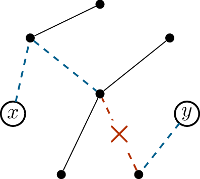
This is why we need to work with two leaves at once. In \(T\), there is an \(x-y\) path \(P\). Change \(H\) to a new graph \(H'\) by toggling every edge along \(P\). That is, for every edge of \(P\), if it is not in \(H\), add it, and if it is in \(H\), remove it. The toggled edges are shown
in Figure 10.5(c), with the final result
\(H'\) shown in Figure 10.5(d).
(In Chapter 14, we will define this as the
symmetric difference operation: \(H' = H \oplus P\). In the meantime, if
the explanation is not clear, rely on Figure 10.5)
We can check by cases that every degree in \(H'\) is odd:
A vertex not in \(V(P\)) is
untouched, and still has odd degree.
Vertices \(x\) and \(y\) gain an edge (because the edges
incident to \(x\) and to \(y\) were not in \(H\) before), so their degree goes from
\(0\) to \(1\): an odd number.
Finally, a vertex in \(V(P)\)
other than \(x\) and \(y\) either gained two edges, gained an edge
and lost an edge, or lost two edges. The change in degree is \(+2\), \(+0\), or \(-2\), so the degree remains odd.
Therefore \(T\) has a spanning
subgraph in which every vertex has odd degree: the subgraph \(H'\). By induction, the same is true
for every tree with an even number of vertices. ◻
Can a tree with an odd number of vertices
have a spanning subgraph such as the one in Proposition 10.8?
No: that would be a graph with an odd
number of vertices, all with odd degree, which cannot exist by
Corollary 4.2 to the
handshake lemma.
This example is also an illustration of an idea that I first
mentioned in Chapter 9: if we must
prove a theorem for connected graphs, and the theorem is only helped by
having more edges, then it’s enough to prove the theorem for trees—which
will be the hardest case.
Here, once we have Proposition 10.8, we
may immediately obtain the following corollary, which was proven by
Atsushi Amahashi in 1985 [3], and later appeared as a problem on the
2005 Bay Area Mathematical Olympiad [7].
Corollary 10.9. Every connected graph with an
even number of vertices has a spanning subgraph (not necessarily
connected) in which every vertex has odd degree.
Proof. Apply Proposition 10.8 to a
spanning tree of the graph. ◻
Practice problems
Let \(T\) be tree whose degree
sequence has the form \(4, 3, 2, 1, 1, 1,
\dots\) (that is, \(4,3,2\)
followed by some number of \(1\)’s).
Determine the number of \(1\)’s
in the degree sequence of \(T\).
There is more than one possibility for a tree \(T\) with this degree sequence. Give two
non-isomorphic trees with this degree sequence, and explain why they are
not isomorphic.
Find all \(6\)-vertex trees up
to isomorphism. (There are six of them.)
Let \(G\) be a graph with \(10\) vertices and \(10\) edges.
If \(G\) contains exactly one
cycle, how many connected components must it have? Give an example of
such a graph.
If \(G\) contains exactly two
cycles, how many connected components must it have? Give an example of
such a graph.
If \(G\) contains exactly three
cycles, there’s two possible values for the number of connected
components. Why is that? Give examples for each possibility.
Prove that when \(n\) is a
multiple of \(3\), there is a solution
to the \(n\times n\) flower garden
problem which contains at least \(\frac23 (n^2
- n) + 2\) flowers.
(You will have to come up with a generalizable layout for the flower
garden which contains this many flowers. See if you can generalize the
layout in Figure 10.1(c).)
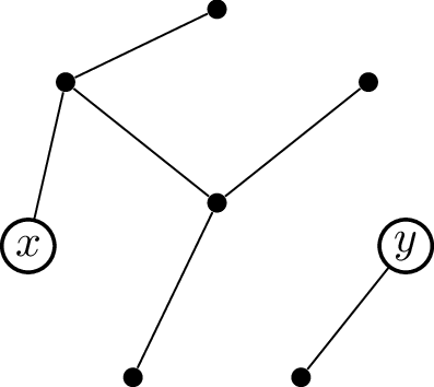
Prove that if \(x\) and \(y\) are vertices of a graph \(G\) in the same connected component, then
adding edge \(xy\) to \(G\) creates at least one new
cycle.
Imitate the proof of Theorem 10.1 to prove that
a graph with \(n\) vertices and \(m\) edges has at least \(m-n+1\) cycles.
Let \(T\) be a weighted tree in
which the cost \(c(e)\) of every edge
is a positive integer. Prove that it’s possible to choose a positive
integer value \(f(x)\) for each vertex
\(x\) such that for all edges \(xy \in E(T)\), \(c(xy) = |f(x) - f(y)|\). An example of
being given such a problem and solving it is shown below:
Find an example of a weighted graph (not a tree!) where every
cost \(c(e)\) is a positive integer,
but the task in part (a) is not possible.
Prove that if \(T\) is a \(k\)-vertex tree and \(G\) is a graph with minimum degree at least
\(k-1\), then \(G\) contains a copy of \(T\).
In Chapter 6, we had
a rather complicated procedure for determining whether there is a graph
with a given degree sequence. If we want to know whether a tree with a
given degree sequence exists, the problem is much easier!
Prove that for any sequence of \(n\ge
2\) positive integers whose sum is \(2(n-1)\), there is a tree with that degree
sequence.
Prove that a \(99\)-vertex tree
cannot have two vertices of degree \(50\).
Let \(T_1\) and \(T_2\) be two trees such that \(T_1 \cap T_2\) (the graph whose vertices
and edges are exactly the vertices and edges present in both \(T_1\) and \(T_2\)) is also a tree. Prove that the union
\(T_1 \cup T_2\) is a tree.
(APMO 2010) Let \(n\) be a
positive integer. \(n\) people take
part in a certain party. For any pair of the participants, either the
two are acquainted with each other or they are not. What is the maximum
possible number of the pairs for which the two are not acquainted but
have a common acquaintance among the participants?
Footnotes
I am going to state the result we get in a more general
form, to allow for the possibility of cycles in the garden path and
unused squares in the garden, but in spirit it is about spanning
trees.↩︎
Later, the ability to prove this result much more easily
will give you a well-deserved feeling of power.↩︎