Cayley's Formula - Start Doing Graph Theory

How to count graphs

Graph enumeration is a whole discipline of graph theory, but we have a lot of ground to cover in this textbook. As a result, this is the first and only chapter in which we will seriously look at problems about counting graphs satisfying a given property.

When we count graphs, we must first choose between two options that are typically described as “counting labeled graphs” and “counting unlabeled graphs”. This is a bit misleading, because all graphs are labeled, in the sense that all graphs have a vertex set with distinguishable elements. Here is how to describe these options more precisely.

Counting labeled graphs is typically the easier of the two problems. To describe it more precisely, suppose that we being by choosing a set \(V\) of size \(n\): it does not matter too much which set \(V\), as long as we choose it, so choosing \(V = \{1, 2, \dots, n\}\) is a very reasonable and simple choice. Then we ask: how many graphs with vertex set \(V\) have a certain property?

The other option is to count graphs up to isomorphism, and this is the problem typically called “counting unlabeled graphs”. Here, we start with the set \(\mathcal S\) of all labeled graphs of that type (again, with some fixed vertex set \(V\)). In most problems, some of the graphs in \(\mathcal S\) will be isomorphic. Graph isomorphism is an equivalence relation on \(\mathcal S\), so it can be used to split \(\mathcal S\) into equivalence classes. When we count graphs up to isomorphism, we ask: how many equivalence classes are there?

In this chapter, we will count \(n\)-vertex trees. Most of the chapter is devoted to the labeled counting problem, for which a clean and beautiful formula exists. Much less is known about the unlabeled counting problem, but I will summarize what is known about it at the end of the chapter.

For either counting problem, one of the most important tools graph theorists use is counting by bijection. If a function \(f\colon X \to Y\) is a bijection, then the sets \(X\) and \(Y\) have the same size: to a set theorist, this is actually how the size of a set is defined. Our bijections will be bijections from a set of graphs to a set of sequences, and so we will think of them somewhat differently: we will call them encoding schemes.

An encoding scheme is a rule by which we can take a graph (or whatever else) and write down a sequence of numbers to represent it. This is a very natural idea in the modern day, when every piece of information has an encoding scheme: after all, a computer must represent all the data it works with as by sequences of zeroes and ones. That’s exactly the way you should think about encoding schemes.

We will want to know two things about our encoding schemes. These correspond to the definition of a bijection, though we won’t invoke that definition directly.

We will want to make sure that the encoding scheme is a unique encoding scheme: from the sequence it produces as an output, we can uniquely determine which graph was the input. It’s nice if we have a simple algorithm to find the graph, but all that’s strictly necessary is to know that two different graphs never produce the same sequence.
We will want to know which sequences of numbers are valid encodings: which ones

An encoding scheme can be described as a function \(f\) from graphs to encodings, and both of the properties above can be phrased in terms of \(f\).

If the encoding scheme is unique, what does that say about \(f\)?

It says that \(f\) is an injective (one-to-one) function.

If every element of some set \(S\) is a valid encoding, what does that say about \(f\)?

It says that \(f\) is a surjective (onto) function, at least if it is a function to the set \(S\).

So that’s the connection to bijections. For our purposes, the consequence is this: once we verify that we have a unique encoding scheme of a set of graphs, we can count the graphs in that set by counting the valid encodings.

To avoid getting too abstract about it, here are two examples.

Problem 11.1. How many graphs with vertex set \(\{1,2,\dots,n\}\) are there?

Answer to Problem 11.1. We will encode these graphs as binary strings of length \(\binom n2\). Here, \(\binom n2 = \frac{n(n-1)}{2}\) is the number of edges in the complete graph \(K_n\) (which we also consider to have vertex set \(\{1,2,\dots,n\}\)). To encode a graph \(G\) with \(V(G) = \{1,2,\dots,n\}\), we go through the edges of \(K_n\) in a fixed order, such as the dictionary order \[12, 13, \dots, 1n, 23, 24, \dots, 2n, \dots.\] For each edge, we ask: does \(G\) also contain that edge? If so, we write down a \(1\); if not, we write down a \(0\).

From the output of this procedure, we can look through the bits one at a time and uniquely determine the edge set \(E(G)\), so this is a unique encoding scheme. Starting from an arbitrary sequence of \(\binom n2\) zeroes and ones, we can reconstruct a graph that will give that sequence, so every one of these sequences is a valid encoding.

There are \(2^{\binom n2}\) sequences of \(\binom n2\) zeroes and ones (because we have \(2\) choices for each bit in the sequence) and therefore there are \(2^{\binom n2}\) graphs with vertex set \(\{1,2,\dots,n\}\). ◻

Problem 11.2. How many \(1\)-regular graphs with vertex set \(\{1,2,\dots,n\}\) are there?

Answer to Problem 11.2. As we know from Chapter 5, such graphs only exist when \(n\) is even. In the cases of even \(n\), we could begin by listing all \(n/2\) edges in the graph. This is done in Figure 11.1 in the case \(n=4\).

Are there multiple ways to list the edges in a graph in a sequence?

Yes: for each edge \(xy\), we can also write it as \(yx\), and we can also write the edges in any order.

To make the encoding scheme unique, we should make a rule for how the edges should be written, and in which order they should appear. A simple option is to write a “sorted sequence of sorted edges”: to sort each edge \(xy\) so that \(x<y\), and to sort the sequence of edges by the first number in each pair. This is already done in Figure 11.1.

Are all “sorted sequences of \(n/2\) sorted edges” valid encodings?

No: some of them encode graphs with \(n/2\) edges that are not \(1\)-regular, by leaving out some vertices and using others too many times. Each vertex must appear exactly once.

If not all sequences are valid encodings, this complicates our life, but we can still proceed. We just have to describe which encodings are valid, and count only the valid ones.

Going from left to right, what are the constraints on the vertices in the “sorted sequence of sorted edges”?

The first vertex of each sorted edge is uniquely determined: it is simply the smallest element of \(\{1,2,\dots,n\}\) that has not yet appeared. The second vertex of each sorted edge can be any of the vertices that have not yet appeared.

How many possibilities are there for each vertices, given the vertices to its left?

There is only \(1\) option for the first vertex of each sorted edge. For the second vertex in the \(k\)^th sorted edge, there are \(n-2k+1\) options, because \(2k-1\) vertices have already appeared.

In such a case, we can count by the product principle, multiplying the numbers of possible vertices in each position. We can do so because that number of options is always the same for a given position, no matter which vertices came before. (Always make sure that this is true before applying the product principle!)

Multiplying together the numbers of possible vertices in each position, we get the product \[\underbrace{1 \cdot (2n-1) \cdot 1 \cdot (2n-3) \cdot 1 \cdot (2n-5) \cdots 1 \cdot 3 \cdot 1 \cdot 1}_{n \text{ factors}}\] in answer to the problem. We can ignore the factors of \(1\) and just say that this is the product of the first \(n/2\) odd positive integers. For example, we get \(3 \cdot 1 = 3\) when \(n=4\) (as seen in Figure 11.1), \(5 \cdot 3 \cdot 1 = 15\) when \(n=6\), \(7\cdot 5 \cdot 3 \cdot 1 = 105\) when \(n=8\), and so on. This product is often written with the double factorial symbol \((2n-1)!!\). ◻

Trees and deletion sequences

Having solved a few problems for practice, we can move on to the question we’re really interested in: how many trees with vertex set \(\{1,2,\dots,n\}\) are there?

The solution to Problem 11.2 gives us a good starting point. An \(n\)-vertex tree, as we know, is in particular an \((n-1)\)-vertex graph. So we can begin by writing down the edges of that graph, in a convenient order.

The most convenient order to use here is not the dictionary order we used before. We would like to make use of the structure of a tree! In particular, we know from Lemma 10.6 in the previous chapter that if we remove a leaf vertex (and its only edge) from a tree, we get a smaller tree. We used this to great effect to write inductive proofs of theorems about trees; it can be used to equally great effect to write recursive algorithms for problems about trees.

Given a tree \(T\) with vertex set \(\{1,2,\dots,n\}\), here is an algorithm to list all its edges in a uniquely defined order:

If \(n=1\), then there are no edges, so the list of edges should be empty as well.
Otherwise, for \(n>1\), the tree \(T\) will have some leaves. Let \(x\) be the lowest numbered leaf, and let \(y\) be its neighbor: write down the pair \((x,y)\), in that order.
Delete vertex \(x\) and edge \(xy\) from \(T\) to get an \((n-1)\)-vertex tree \(T-x\). To write the rest of the sequence, go back to step 1, but with tree \(T-x\) in place of \(T\).

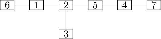
We will call the result of this algorithm a deletion sequence¹ for \(T\). As an illustration of the technique, Figure 11.2 shows how, starting with the tree in Figure 11.2(a), we determine that its deletion sequence is \[(1,4),\; (3,4),\; (4,6),\; (5,2),\; (6,2),\; (2,7).\]

Is this a unique encoding scheme?

Yes, it is. We can recover the tree from its deletion sequence, because the deletion sequence is after all a list of edges. Moreover, each tree only has one deletion sequence, because the deletion sequence is computed by an algorithm with no freedom at any step.

There is a great deal of redundancy in the deletion sequence of a tree. Before proving a general result about it, let’s explore a few examples. In all of these, I will erase some numbers from the deletion sequence we just constructed and ask how they can be filled back in to get a valid deletion sequence. Of course, one way to fill in the number is to put back the number we erased, getting back the deletion sequence we started with. However, we want to know if there are any other deletion sequences that have a different value in that blank!

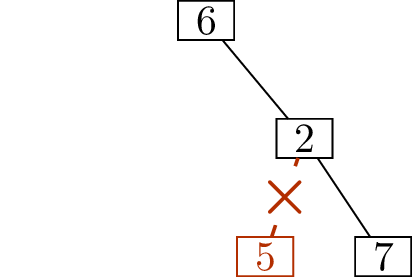
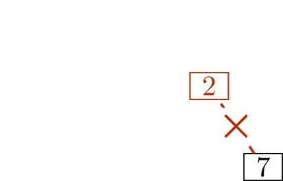
In the incomplete deletion sequence \[(1,4),\; (3,4),\; (4,6),\; (5,2),\; (6,2),\; (2,\underline{\phantom{7}}),\] how many ways are there to fill in the blank?

The number in the blank can only be \(7\).

The reason is that vertex \(7\) will never be deleted as the smallest leaf of the tree: there are always at least two leaves, one of which is smaller than \(7\). Therefore it is the last vertex remaining, and will always occupy the last position in the deletion sequence.

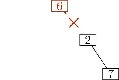
In the incomplete deletion sequence \[(1,4),\; (3,4),\; (\underline{\phantom{4}},6),\; (5,2),\; (6,2),\; (2,7),\] how many ways are there to fill in the blank?

The number in the blank can only be \(4\).

The reason is that vertices \(1, 2, 3, 4, 5, 6\) must all be eventually deleted. The five complete ordered pairs tell us when we deleted vertices \(1\), \(2\), \(3\), \(5\), and \(6\), so the incomplete ordered pair must tell us when we deleted vertex \(4\).

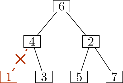
In the incomplete deletion sequence \[(1,4),\; (3,4),\; (\underline{\phantom{4}},6),\; (\underline{\phantom{5}},2),\; (6,2),\; (2,7),\] how many ways are there to fill in the two blanks?

Once again, the answer is uniquely determined: the blanks must contain \(4\) and \(5\), in that order.

By the same reasoning as above, we know that \(4\) and \(5\) must go in those two blanks in some order. Since neither number appears later in the deletion sequence, we know that none of their neighbors are deleted later: after the first two steps, both vertices \(4\) and \(5\) are leaves. Since \(4\) is a smaller number, it will be the leaf deleted first.

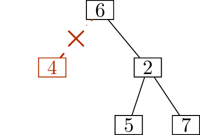
But all of these questions are thinking too small: we can take the incomplete sequence \[(\underline{\phantom{1}},4),\; (\underline{\phantom{3}},4),\; (\underline{\phantom{4}},6),\; (\underline{\phantom{5}},2),\; (\underline{\phantom{6}},2),\; (\underline{\phantom{2}},\underline{\phantom{7}})\] and fill in all \(7\) blanks in a unique way!

First of all, we know that the first six blanks are the numbers \(1\) through \(6\), while the last blank is \(7\). The order of the numbers \(1\) through \(6\) is not known yet, but even without knowing the order, we know how many times each number appears in the deletion sequence, in total: the number of times we see it in the incomplete sequence, plus \(1\).

This tells us the degree of every vertex: \[\begin{array}{c|ccccccc} x & 1 & 2 & 3 & 4 & 5 & 6 & 7 \\ \hline \deg(x) & 1 & 3 & 1 & 3 & 1 & 2 & 1 \end{array}\] Why is this helpful? Because it tells us that at the beginning of the algorithm to generate the deletion sequence, the leaves were \(1\), \(3\), \(5\), and \(7\). Of these, \(1\) is the smallest, so it must be the first leaf deleted: the first pair is \((1,4)\).

From there, we can deduce that after vertex \(1\) is deleted, the degrees of the vertices were as follows: \[\begin{array}{c|cccccc} x & 2 & 3 & 4 & 5 & 6 & 7 \\ \hline \deg(x) & 3 & 1 & 2 & 1 & 2 & 1 \end{array}\] The leaves were \(3\), \(5\), and \(7\), of which \(3\) is the smallest. Therefore the second pair must be \((3,4)\).

If we keep going in this manner, we can reconstruct the entire deletion sequence, because we can determine the degree of each remaining vertex at each step of the algorithm. Only \(5\) of the \(12\) numbers in the deletion sequence were necessary!

Prüfer codes

Our strategy in the preceding section generalizes fully. We can summarize the properties we use in the following two properties of a deletion sequence \((a_1, b_1), (a_2, b_2), \dots, (a_{n-1}, b_{n-1})\):

For every \(k\) from \(1\) to \(n-1\), the number \(a_k\) is the smallest positive number not contained in the set \(\{a_1, a_2, \dots, a_{k-1}\} \cup \{b_k, b_{k+1}, \dots, b_{n-2}\}\).
\(b_{n-1}=n\).

Lemma 11.1. If a sequence \((a_1, b_1), (a_2, b_2), \dots, (a_{n-1}, b_{n-1})\) is the deletion sequence of a tree with vertices \(1, 2, \dots, n\), then it satisfies properties (1) and (2).

Proof. The tree at every stage of the algorithm that generates the deletion sequence has at least two leaves, so the smallest leaf will never be vertex \(n\). Therefore vertex \(n\) will never be the deleted leaf, so it will be the last vertex remaining: \(b_{n-1} = n\). This proves (2).

Meanwhile, \(a_1, \dots, a_{n-1}\) are a permutation of \(1, 2, \dots, n-1\), representing the order in which the other vertices are deleted. After the first \(k-1\) stages of the algorithm that generates the deletion sequence, the tree that remains has edges \((a_k, b_k)\) through \((a_{n-1}, b_{n-1})\). Vertices in the set \(\{a_1, a_2, \dots, a_{k-1}\}\) are not present in this tree; they have already been deleted.

The remaining vertices of the tree appear once in the set \(\{a_k, a_{k+1}, \dots, a_{n-1}, b_{n-1}\}\). They have degree \(1\) if this is their only appearance: if they do not appear in the set \(\{b_k, b_{k+1}, \dots, b_{n-2}\}\). Vertex \(a_k\) is the smallest leaf remaining at this stage, so it is the smallest positive number not contained in the set \(\{a_1, a_2, \dots, a_{k-1}\} \cup \{b_k, b_{k+1}, \dots, b_{n-2}\}\). This proves (1). ◻

Since the numbers determined by Lemma 11.1 can be deduced from the others, they are not necessary to recover the tree. Therefore, instead of recording the deletion sequence of a tree, it is enough to record the sequence \((b_1, b_2, \dots, b_{n-2})\). This sequence is called the Prüfer code of the tree, named after Heinz Prüfer, who proposed Prüfer codes as a method of counting labeled trees in 1918 [87].

It is worth mentioning that the Prüfer code of a tree can be directly computed using an abbreviated version of the algorithm that computed the deletion sequence. The only two differences are that instead of writing down the pair \((x,y)\), we only write down the vertex \(y\), and that we stop when there are \(2\) vertices and \(1\) edge left. Figure 11.3 illustrates this on an example.

Are Prüfer codes a unique encoding scheme?

Yes: from the Prüfer code, we can recover the deletion sequence using properties (1) and (2), and the deletion sequence simply tells us the edges of the tree.

Is this enough to count the with vertex set \(\{1,2,\dots,n\}\)?

No: we need to know whether all possible sequences \((b_1, b_2, \dots, b_{n-2})\) are valid Prüfer codes, or whether there are some constraints on these numbers.

In fact, there are no further constraints: every sequence \((b_1, b_2, \dots, b_{n-2})\), where each term is an element of \(\{1,2,\dots,n\}\), is the Prüfer code of a tree with vertex set \(\{1,2,\dots,n\}\). To prove this, the most important claim we have not yet shown is that (1) and (2) are not just properties every deletion sequence has: they are properties only a deletion sequence can have.

Lemma 11.2. If a sequence \((a_1, b_1), (a_2, b_2), \dots, (a_{n-1}, b_{n-1})\) in which every term \((a_i, b_i)\) is a pair of numbers from \(1\) to \(n\) satisfies properties (1) and (2), then it is the deletion sequence of a tree with vertex set \(\{1,2,\dots,n\}\).

Proof. Let’s make some initial observations. First, since \(a_k \notin \{a_1, a_2, \dots, a_{k-1}\}\), the numbers \(a_1, a_2, \dots, a_{n-1}\) are distinct. They are all smaller than \(n\), since each is the smallest positive number not contained among at most \(n-2\) options; therefore, they are a permutation of \(\{1,2,\dots,n-1\}\).

Second, consider \(b_k\) for \(1 \le k \le n-2\). Since none of \(a_1, a_2, \dots, a_k\) can equal \(b_k\), but \(b_k\) is an integer from \(1\) to \(n\), we know that it must be an element of \(\{a_{k+1}, \dots, a_{n-1}, n\}\). From this observation, it follows that we can define a graph \(T_k\) with \(V(T_k) = \{a_k, a_{k+1}, \dots, a_{n-1}, n\}\) and \(E(T_k) = \{a_k b_k, a_{k+1}b_{k+1}, \dots, a_{n-1}b_{n-1}\}\): each edge in \(E(T_k)\) really does have both endpoints in \(V(T_k)\).

We are now ready to proceed with the proof. The graph \(T_k\) is not just any graph: it is a tree in which the leaf with the smallest number is \(a_k\). We will prove this by an induction that starts with \(T_{n-1}\) and ends with \(T_1\).

In the base case, \(T_{n-1}\) is the graph with vertices \(\{a_{n-1}, n\}\) and edge \(a_{n-1} b_{n-1}\); since \(b_{n-1}=n\), this is an edge between \(T_{n-1}\)’s two vertices, so \(T_{n-1}\) is a tree. Both \(a_{n-1}\) and \(b_{n-1}\) are leaves, but since \(b_{n-1}=n\) and \(a_{n-1} \ne b_{n-1}\), \(a_{n-1}\) must be the smaller leaf.

Next, for some positive \(k<n-1\), suppose \(T_{k+1}\) is a tree. The only difference between \(T_k\) and \(T_{k+1}\) is that we add vertex \(a_k\) and edge \(a_k b_k\). By our first observation, \(a_k \notin V(T_{k+1})\), so \(a_k\) is a leaf of \(T_k\). Since \(T_{k+1}\) is a tree, it has no cycles, so \(T_k\) cannot contain any cycles not using vertex \(a_k\). It cannot have any cycles using \(a_k\), either, because \(a_k\) has degree \(1\). Therefore \(T_k\) still has no cycles; we know it has \(n-k+1\) vertices and \(n-k\) edges, so it is a tree by condition 5 of Theorem 10.2.

Each \(a_i\) for \(i<k\) is not yet a vertex of \(T_k\), by our first observation. Each \(b_i\) for \(i\ge k\) appears a second time as \(a_j\) for \(j>i\), by our second observation; so it is the endpoint of at least two edges of \(T_k\), and is not a leaf. Among the remaining positive integers, \(a_k\) is the smallest; therefore in particular it is the smallest leaf of \(T_k\). This completes the induction.

From this claim, it follows that the deletion sequence algorithm, when encountering tree \(T_k\), will write down the pair \((a_k, b_k)\) and delete \(a_k\), then either go on to tree \(T_{k+1}\) or (if \(k=n-1\)) stop. In particular, if we start with tree \(T_1\), the deletion sequence algorithm will proceed through the trees \(T_2, T_3, \dots, T_{n-1}\) and write down the sequence \[(a_1, b_1), (a_2, b_2), \dots, (a_{n-1}, b_{n-1}),\] which is exactly what we wanted to show. ◻

With this setup complete, we are ready to finish counting. This theorem is known as Cayley’s formula after Arthur Cayley, whom we already know as the mathematician that came up with the term “tree”. (So, you see, Prüfer’s argument was not the first to be found. However, as it sometimes happens, Cayley was not the first, either; the formula was first proven by Carl Wilhelm Borchardt in 1860 [9].)

Theorem 11.3. There are \(n^{n-2}\) trees with vertex set \(\{1,2,\dots,n\}\).

Proof. Each tree with vertex set \(\{1,2,\dots,n\}\) has a Prüfer code \((b_1, b_2, \dots, b_{n-2})\) whose elements are integers between \(1\) and \(n\), uniquely defined by the deletion sequence algorithm. Therefore the number of trees with vertex set \(\{1,2,\dots,n\}\) is exactly the number of possible Prüfer codes.

Moreover, for every such sequence \((b_1, b_2, \dots, b_{n-2})\), we can apply (1) to determine \(a_1\), then \(a_2\), and so on through \(a_{n-1}\), as long as we go in that order: each \(a_k\) will be the smallest positive integer not contained in a set we’ve already entirely determined. We can also set \(b_{n-1} = n\). Now, the sequence \[(a_1, b_1), (a_2, b_2), \dots, (a_{n-1}, b_{n-1})\] is a deletion sequence of a tree with vertex set \(\{1,2,\dots,n\}\), by Lemma 11.2, and therefore \((b_1, b_2, \dots, b_{n-2})\) is the Prüfer code of that tree. This shows that every sequence \(n-2\) integers from \(1\) to \(n\) is a valid Prüfer code. There are exactly \(n^{n-2}\) such sequences, since there are \(n\) options for each of the numbers \(b_1\) through \(b_{n-2}\), so the number of trees with vertex set \(\{1,2,\dots,n\}\) is also \(n^{n-2}\). ◻

Working with Prüfer codes

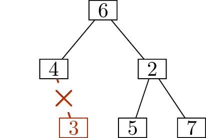
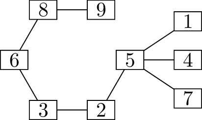
There are a few more difficult questions to ask about Prüfer codes, but let’s first pause to make sure that we can return from the abstract results to concrete claims. Take a Prüfer code like \((2,1,2,5,4)\). How do we turn it back into a tree?

Let’s write down what we know about the deletion sequence of that tree, even if there’s still some blanks to be filled in: \[(\underline{\phantom{0}}, 2), (\underline{\phantom{0}}, 1), (\underline{\phantom{0}}, 2), (\underline{\phantom{0}}, 5), (\underline{\phantom{0}}, 4), (\underline{\phantom{0}}, \underline{\phantom{0}}).\] A Prüfer code is always a sequence of \(n-2\) numbers from \(1\) to \(n\); since we started with \(5\) numbers, their values will range from \(1\) to \(7\). We fill in the blanks from left to right.

For the first blank, which is \(a_1\), we use (1). There are no \(a\)-terms before \(a_1\); however, \(a_1\) needs to be distinct from \(\{b_1, b_2, b_3, b_4, b_5\} = \{1, 2, 4, 5\}\). The smallest integer not on this list is \(3\), so we set \(a_1 = 3\): \[(3, 2), (\underline{\phantom{0}}, 1), (\underline{\phantom{0}}, 2), (\underline{\phantom{0}}, 5), (\underline{\phantom{0}}, 4), (\underline{\phantom{0}}, \underline{\phantom{0}}).\] We continue to use (1) for the next blank, which is \(a_2\). Here, the excluded values are \(a_1, b_2, b_3, b_4, b_5\) or \(3, 1, 2, 5, 4\). We fill in the blank with the first integer not on this list, which is \(6\): \[(3, 2), (6, 1), (\underline{\phantom{0}}, 2), (\underline{\phantom{0}}, 5), (\underline{\phantom{0}}, 4), (\underline{\phantom{0}}, \underline{\phantom{0}}).\] We go on in this way. Some people prefer to arrange the entries in a \(2 \times (n-1)\) table, where each \(a_i\) entry (in the first, initially empty row) must be distinct from everything to its left, as well as everything below it and to the right: \[\begin{array}{c|c|c|c|c|c} a_1 & a_2 & a_3 & a_4 & a_5 & a_6 \\ \hline b_1 & b_2 & b_3 & b_4 & b_5 & b_6 \end{array} \quad = \quad \begin{array}{c|c|c|c|c|c} 3 & 6 & ? & & & \\ \hline 2 & 1 & 2 & 5 & 4 & \end{array}\] Regardless, we fill in \(a_3 = 1\) (the smallest value not among \(3, 6, 2, 5, 4\)), then \(a_4 = 2\) (the smallest value not among \(3, 6, 1, 5, 4\)), then \(a_5 = 5\) (the smallest value not among \(3, 6, 1, 2, 4\)), then \(a_6 = 4\) (the smallest value not among \(3, 6, 1, 2, 5\)). All this is done using (1); then, the last blank is \(b_6 = 7\) by (2). The completed deletion sequence is \[(3, 2), (6, 1), (1, 2), (2, 5), (5, 4), (4, 7).\] This sequence tells us the edges of the tree, and if we like, we can draw a diagram such as the one in Figure 11.4.

The tree with Prüfer code \((2, 1, 2, 5, 4)\).

That being said, it is not too often that we find ourselves needing to actually convert a Prüfer code back into a tree: it only matters for the proof of Theorem 11.3 that we can, in principle, do it.

This does not mean that Prüfer codes have no use beyond the proof of Theorem 11.3. The Prüfer code of a tree actually contains a bit of information about the tree, which we can use to solve more complicated counting problems. For example:

Proposition 11.4. In the Prüfer code of a tree where \(\deg(x) = k\), the number \(x\) appears \(k-1\) times.

Proof. When we fill in the blanks in the sequence \[(\underline{\phantom{a_1}}, b_1), (\underline{\phantom{a_1}}, b_2), \dots, (\underline{\phantom{a_1}}, b_{n-2}), (\underline{\phantom{a_1}}, \underline{\phantom{a_1}})\] we use each of the numbers \(1, 2, \dots, n\) once. The number \(n\) is going to fill in the second blank of the last pair, and the numbers in the first blanks are a permutation of \(1, 2, \dots, n-1\).

Therefore if a number \(x\) appears \(k-1\) times in the Prüfer code, it appears \(k\) times in the deletion sequence \[(a_1, b_1), (a_2, b_2), \dots, (a_{n-1}, b_{n-1}).\] But the deletion sequence is just a particular way to write down the edges of the tree, so if \(x\) appears in the deletion sequence \(k\) times, then it is the endpoint of \(k\) edges, which is just another way of saying that \(\deg(x) = k\). ◻

For example, even before we turned the Prüfer code \((2,1,2,5,4)\) back into the tree shown in Figure 11.4, we could have known the rough structure of the tree:

Vertices \(3\), \(6\), and \(7\) are leaves, because they do not appear in the Prüfer code at all.
Vertices \(1, 4, 5\) appear once, and therefore have degree \(2\).
Vertex \(2\) appears twice, and therefore has degree \(3\).

What can we say about the shape of such a tree, knowing only the degrees of the vertices?

Such a tree must consist of three paths starting at vertices \(3\), \(6\), \(7\) and converging at vertex \(2\).

Here is a quick example of using Proposition 11.4 to solve a counting problem:

Corollary 11.5. There are \((n-1)^{n-2}\) trees with vertex set \(\{1, 2, \dots, n\}\) in which vertex \(1\) is a leaf.

Proof. By Proposition 11.4, vertex \(1\) is a leaf (has degree \(1\)) if and only if the number \(1\) never appears in the Prüfer code. There are \((n-1)^{n-2}\) such codes: the code is a sequence with \(n-2\) terms, each of which is now restricted to one of the \(n-1\) values in the set \(\{2, 3, \dots, n\}\). Therefore there are \((n-1)^{n-2}\) such trees. ◻

Unlabeled trees

Now that we’ve counted labeled trees on \(n\) vertices, we can try to say something about unlabeled trees. How many \(n\)-vertex trees are there, up to isomorphism? As I mentioned earlier in this chapter, we can think of this as counting equivalence classes of the \(n^{n-2}\) trees with vertex set \(\{1,2,\dots,n\}\). Each equivalence class is a set of trees that are isomorphic (but not equal).

Sometimes, if we’re very lucky, the equivalence classes all have the same size. In that case, to count the equivalence classes, we can divided by the number of elements of one equivalence class. Let’s begin by destroying all such hopes: when we count trees, the equivalence classes are far from equal in size.

Figure 11.5(a) shows the path graph \(P_n\). How many trees with vertex set \(\{1,2,\dots,n\}\) are isomorphic to it?

There are \(n!\) ways to put the vertices in order from left to right along the path. However, the graph does not know a “left” and a “right”: if you reverse the sequence, you get the same graph, drawn in reverse. Therefore there are \(\frac 12 n!\) paths with vertex set \(\{1,2,\dots,n\}\).

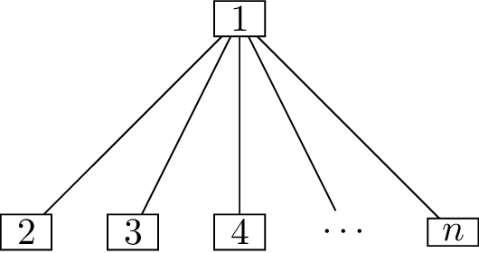
Figure 11.5(b) shows the star graph \(S_n\). How many trees with vertex set \(\{1,2,\dots,n\}\) are isomorphic to it?

As soon as we choose which vertex in the set \(\{1,2,\dots,n\}\) is the vertex of degree \(n-1\) at the center of the star, the graph is completely determined. Therefore there are \(n\) stars with vertex set \(\{1,2,\dots,n\}\).

If all \(n\)-vertex trees were like \(P_n\), then every equivalence class would have \(\frac12 n!\) elements, and the number of equivalence classes would be the quotient \(n^{n-2}/(\frac12 n!)\). If instead all \(n\)-vertex trees were like \(S_n\), then every equivalence class would have \(n\) elements, and the number of equivalence classes would be \(\frac{n^{n-2}}{n}\) or \(n^{n-3}\).

In reality, neither of these extremes is the case. The truth is somewhere in the middle; but it is more like the first answer than the second. Why? Well, the reason that there are very few different trees isomorphic to \(S_n\) is that the star graph has a lot of symmetry. Most large trees are not nearly as symmetric, so most equivalence classes are pretty large.

A result known as Stirling’s formula says that, very approximately, \(n!\) grows like \((\frac ne)^n\), where \(e \approx 2.718\) is Euler’s number.² If we plug this into the quotient \(n^{n-2}/(\frac12 n!)\), we get an estimate of \(2e^n/n^2\) for the number of unlabeled trees. This is not the true growth rate, but it is the right type of growth: the number of unlabeled trees really does grow exponentially. That growth rate was first precisely analyzed in 1937 by George Pólya [83], who described it as an exponential \(c^n\) with \(c \approx 2.9557\), divided by a polynomial factor.

No exact formula is known. In the Online Encyclopedia of Integer Sequences, the number of \(n\)-vertex unlabeled trees can be found in one of the very first sequences: sequence A000055 [78]. The first few terms are \[1, 1, 1, 1, 2, 3, 6, 11, 23, 47, 106, 235, \dots\] The initial \(1\)’s in this sequence correspond to \(n=0\)³ through \(n=3\), where only one \(n\)-vertex tree is possible. (For \(n=4\), we have two options: the \(4\)-vertex path, and the \(4\)-vertex star.)

Practice problems

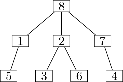
Find the trees with the following Prüfer codes:
1. \((3, 3, 3, 3, 3)\).
2. \((2, 7, 1, 5, 4, 6)\).
3. \((3, 1, 4, 1, 5, 9, 2)\).
Find the Prüfer codes of the following trees:

(One of these Prüfer codes gives you my birth date. Another is the first few digits of Euler’s number \(e\). Another tells you the phone number to call to reach Ghostbusters.)
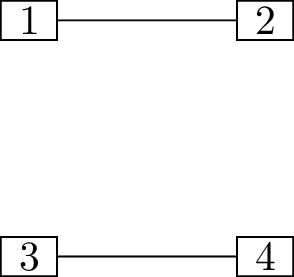
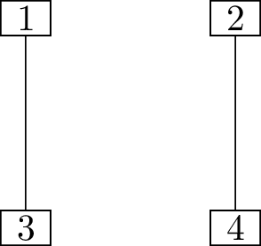
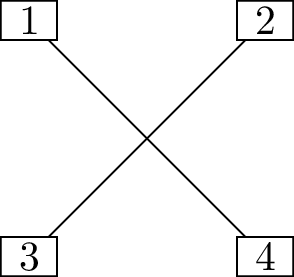
Find all \(16\) trees with vertices \(\{1, 2, 3, 4\}\).
What is the Prüfer code of the path graph in Figure 11.5(a), and what is the general form of a Prüfer code for a tree isomorphic to it?
What is the Prüfer code of the star graph in Figure 11.5(b), and what is the general form of a Prüfer code for a tree isomorphic to it?
Use Prüfer codes and Proposition 11.4 to count:
1. The number of trees with vertex set \(\{1, 2, \dots, n\}\) in which vertex \(1\) has degree \(3\).
2. The number of trees with vertex set \(\{1, 2, \dots, n\}\) in which vertex \(1\) has degree \(n-2\).
3. The number of trees with vertex set \(\{1, 2, \dots, n\}\) in which all vertices except vertex \(1\) and \(2\) have degree \(1\).
For parts (b) and (c), think about how you would count them without using Prüfer codes.
Use Corollary 11.5 to find the average number of leaves in an \(n\)-vertex tree.
Prove that if a tree has maximum degree \(d\), then it has at least \(d\) leaves:
1. Using Prüfer codes and Proposition 11.4.
2. Using ideas from Chapter 10.
Is it true that if only one number is changed in a Prüfer code, then this only changes the tree it corresponds to by one edge?

If so, prove it. If not, find (in terms of \(n\)) the maximum number of edges that can change in the tree, if the Prüfer code changes in only one position.
Let \(f(n)\) be the number of trees with vertex set \(\{1,2,\dots,n\}\) that contain the edge \(12\).
1. Prove that \(f(n)\) is also the number of trees with vertex set \(\{1,2,\dots,n\}\) that contain the edge \(xy\), for any other edge \(xy\) that such a tree could have.
2. Using part (a), find and prove a formula for \(f(n)\).
3. Let \(G\) be a graph with \(n\) vertices and \(\binom n2 - 1\) edges. In terms of \(n\), find the number of spanning trees \(G\) has.

Footnotes

This is not a universally recognized term, but simply the term I will use in this chapter to explain our counting strategy.↩︎
See the second problem at the end of this chapter if you want to know more digits of this constant, but prepare to do some work, first.↩︎
I actually disagree with the OEIS on the initial value; I do not believe there is a \(0\)-vertex tree. Even if we allow \(0\)-vertex graphs to be exist, they would surely have \(0\) edges, but an \(n\)-vertex tree should have \(n-1\) edges. My opinion, which does not really affect anything but definitions and initial terms, is that the \(0\)-vertex graph exists but is not connected.↩︎

Cayley’s formula

The purpose of this chapter