Most graph theory textbooks present the graphic sequence algorithm
differently, by working with numerical sequences rather than directly
with graphs. In my opinion, that makes the problem harder as well as
more boring. This leaves much less class time for discussing edge swaps
and the ideas in the proof of the Havel–Hakimi theorem (Theorem 6.2).
I think that Problem 6.1 and its solution for
\(8\) people is a good way to motivate
the graphic sequence algorithm. The proof of Proposition 6.1 could be skipped in a graph
theory course covering this material, but I felt that I had to include
it to avoid leaving the problem without a solution.
An unusual party
Let me tell you a story.1 One time, I was at a
very large party—there were \(100\)
people there! Not everybody knew each other, of course. In fact, each
person at the party knew a different number of people. In addition,
I—
“—That can’t be right!” you interrupt. “You’re saying that the graph
which represents who knew each other at the party had the degree
sequence \(99, 98, 97, \dots, 2, 1,
0\)? But that’s not a graphic sequence!”
Why isn’t this sequence graphic?
The vertex of degree \(99\) is adjacent to every other vertex, but
the vertex of degree \(0\) is adjacent
to none of the other vertices, and these facts contradict each
other.
Oh, sorry. My mistake. Let me try again.
Problem 6.1. One time, I was at a very large
party—there were \(100\) people there!
Not everybody knew each other, of course. In fact, each person at the
party knew a different number of people, with one exception: I
personally knew the same number of people as another guest, named Masha.
In addition, I can promise you that everyone at this party knew at least
one other person.
Now, given this information, can you tell me how many people I
knew at the party? Also, can you tell me whether Masha and I knew each
other?
Before we solve this problem, let’s consider a smaller case: an \(8\)-person party and its graph of who knows
whom. In this graph, the vertex degrees are \(7, 6, 5, 4, 3, 2, 1\), but with one of
these duplicated. We can’t duplicate an odd number, because then the sum
of degrees would be odd, in violation of Corollary 4.2 to the
handshake lemma. So we must duplicate the \(6\), the \(4\), or the \(2\). I can tell you the correct option:
duplicating the \(4\) is the only
choice that will work.
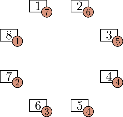
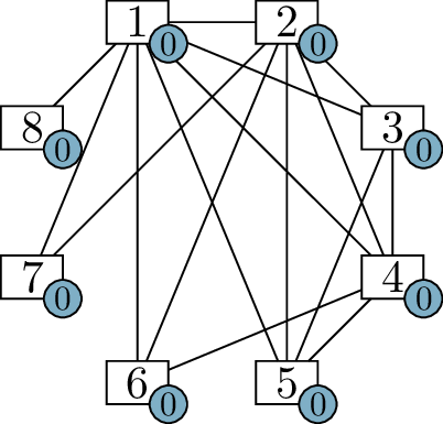
If the degree sequence is \(7, 6, 5, 4, 4,
3, 2, 1\), can we reconstruct the graph? Let me show you a way to
think about it with the aid of a diagram. In Figure 6.1(a), I have drawn vertices \(1\) through \(8\), each with an extra label: the degree
that the vertex wants to have. As we work on filling in the graph, we
will update these labels to show the remaining number of incident edges
that the vertex wants, but doesn’t have yet.
The initial problemStep 1Step 2
Step 3Step 4
Reconstructing the \(8\)-person party
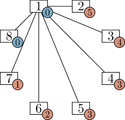
For one of these vertices, we can immediately assign the neighbors.
Vertex 1 needs to be adjacent to every other vertex, so we can draw all
of those edges, as shown in Figure 6.1(b).
This reduces the label on vertex 1 by \(7\) (we’ve given it \(7\) more incident edges), and the label on
each other vertex by \(1\) (we’ve given
each of them \(1\) incident edge). It’s
important to point out that vertex \(1\) and \(8\) now want \(0\) more edges, so they will not be used
again.
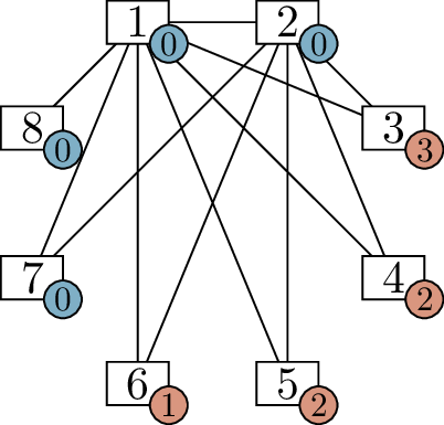
We can continue. Vertex 2 needs \(5\) more edges, and there are only \(5\) other vertices that can accept edges,
so it must be adjacent to all of them! We add all of those edges in
Figure 6.1(c). Updating the label on each
vertex, we see that vertices 2 and 7 are also satisfied.
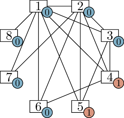
Two more steps solve the problem entirely. When we process vertex
\(3\) in Figure 6.1(c), we arrive at the diagram in
Figure 6.1(d). At that point, we only have
two vertices left to deal with: vertices \(4\) and \(5\). Each one wants \(1\) more neighbor, so we make them
adjacent, arriving at the diagram in Figure 6.1(e). Now we
know all the edges of the graph.
We will return to the ideas in this solution very soon. For now, let
me make one more observation. In Figure 6.1(b),
there are \(6\) vertices left to deal
with (vertices \(2\) through \(7\)), and they demand \(5, 4, 3, 3, 2, 1\) additional edges
respectively. This is a \(6\)-vertex
version of the same problem, which suggests a solution to Problem 6.1 by induction.
Proposition 6.1. For all \(n\ge 1\), up to isomorphism, there is a
unique \(2n\)-vertex graph which
contains a vertex of every degree \(1, 2,
\dots, 2n-1\). In that graph, there are two vertices of
degree \(n\), and they are
adjacent.
Proof. We induct on \(n\).
When \(n=1\), the graph we are looking
for is a graph with \(2\) vertices, at
least one of which has degree \(1\).
There must be an edge between the \(2\)
vertices, and this already describes the graph uniquely. In this graph,
there are two vertices of degree \(1\),
and they are adjacent, completing the base case.
Next, for some \(n>1\), assume
that the previous case of the proposition holds. That is, there is a
unique \(2(n-1)\)-vertex graph \(G\) which contains a vertex of degree \(1, 2, \dots, 2n-3\). In \(G\), there are two vertices of degree \(n-1\), and they are adjacent.
Mimicking the way in which the \(6\)-person party sits inside the \(8\)-person party in Figure 6.1(b), we extend \(G\) to a \(2n\)-vertex graph \(H\) by adding two vertices \(x\) and \(y\); we make \(x\) adjacent to \(y\) and to all vertices of \(G\), and we make \(y\) adjacent only \(x\). Here, \(\deg_{H}(x) = 2n-1\) and \(\deg_{H}(y)=1\); for all vertices \(z \in V(G)\), we have \(\deg_H(z) = \deg_G(z) + 1\) (because we
added the edge \(xz\)) and so the
vertices of \(G\) fill in the degrees
\(2, 3, \dots, 2n-2\). The two vertices
of degree \(n-1\) in \(G\) become vertices of degree \(n\) in \(H\), and they are adjacent.
This proves that the situation in Proposition 6.1 is possible, but not that
it is unique. To prove it is unique, let \(H'\) be any \(2n\)-vertex graph that satisfies the
conditions. Let \(x\) be a vertex of
degree \(2n-1\) in \(H'\), and let \(y\) be a vertex of degree \(1\) in \(H'\). Then \(x\) must be adjacent to all other vertices
(including \(y\)), which means \(y\) is only adjacent to \(x\). Let \(G'
= H' - x - y\); then in \(G'\), every degree \(k\) between \(1\) and \(2n-3\) is present, because degree \(k+1\) is present in \(H\) on a vertex that’s neither \(x\) nor \(y\). Since \(G'\) satisfies the conditions in the
proposition, it must be isomorphic to the graph \(G\) in the previous paragraph, which forces
\(H'\) to be isomorphic to the
graph \(H\) in the previous
paragraph.
How do we know every isomorphism between
\(G\) and \(G'\) extends to an isomorphism between
\(H\) and \(H'\)?
To extend an isomorphism \(\varphi\colon V(G) \to V(G')\), just
define \(\varphi(x)=x\) and \(\varphi(y)=y\). Since in both \(H\) and \(H'\), \(x\) is adjacent to every vertex and \(y\) is adjacent only to \(x\), the extended \(\varphi\) is guaranteed to preserve the
edges out of \(x\) and \(y\).
This proves uniqueness, which completes the induction step; by
induction, the graph exists and is unique up to isomorphism for all
\(n\). ◻
In particular, the answer to Problem 6.1 (the \(n=50\) case of Proposition 6.1) is that Masha and I both
knew \(50\) people at the party, and we
did know each other.
A graphic sequence algorithm
The reconstruction in Figure 6.1 is
only possible for very special degree sequences. Our decision at each
step was forced, and the reason it was forced is the uniqueness result
in Proposition 6.1. Most degree sequences do
not have a corresponding uniqueness result, in which case, life is more
complicated.
What do we do if we’re faced with a diagram like one of the ones in
Figure 6.1, but there are no forced
deductions to make? It turns out that there’s still something we can do.
It will feel like making a lucky guess. Later in this chapter, in
Theorem 6.2, we will prove that the guess
is always justified, at least in one sense. Before we do that, though,
let me explain the guess and why it is at least reasonable.
My reasoning is this: in Figure 6.1, we
were always living life on the edge. The highest-degree vertex always
just barely had enough edges we could place, and that’s why the result
was unique. We would like our graphs to be as little like that,
actually: we want to avoid having vertices which need many edges. We
also want to avoid creating too many inactive vertices (which don’t need
any more edges) too quickly.
Putting these together, which vertex should we deal with next, at
each step? It should be the vertex which is most in danger: the vertex
with the highest remaining degree. Which neighbors should we give it, if
we have the choice? It should be the other vertices with the highest
remaining degree—this ensures those vertices need fewer edges later, and
also avoids creating inactive vertices too early.
Now, let me present an algorithm which makes all these ideas formal
and precise.
Given a sequence of nonnegative integers \(d_1, d_2, \dots, d_n\), our goal is to test
if the sequence is graphic, and if it is, to construct a graph whose
degree sequence is \(d_1, d_2, \dots,
d_n\). We begin our construction with a graph \(G\) that has vertex set \(V(G) = \{1, 2, \dots, n\}\) and edge set
\(E(G) = \varnothing\): no edges to
start with. We will add edges to \(G\)
as we go.
For all \(i=1, \dots, n\), we intend
for vertex \(i\) to have degree \(d_i\) at the end. We give vertex \(i\) a demand representing how many
more edges it needs to meet this goal. Initially, we set its demand
equal to \(d_i\), but we will update
the demand of \(i\) over the course of
the algorithm. We will call a vertex active if its demand is
positive, and inactive if its demand is \(0\). In diagrams, I will give each vertex
an extra label showing its demand.
We repeat the algorithm below for as long as any active vertices
remain. In each iteration, we perform the following steps:
Pick a vertex \(x\) with the
highest possible demand, breaking ties arbitrarily; let \(k\) be the demand of \(x\).
If there are fewer than \(k\)
active vertices other than \(x\), stop
and declare that the sequence is not graphic: we have failed to
construct a graph with this sequence.
Otherwise, let \(S\) be a set of
\(k\) active vertices, other than \(x\), whose demand is as high as possible
(again, breaking ties arbitrarily).
Add the \(k\) edges \(xy\) for all \(y
\in S\) to the graph \(G\). Set
the demand of \(x\) to \(0\) (making it inactive) and decrease the
demand of each vertex \(y \in S\) by
\(1\).
Once no more active vertices remain, we stop.
What is the maximum number of iterations
we will need?
Since at least one vertex becomes inactive
at each step, we can be be certain to stop after \(n\) iterations (in an \(n\)-vertex graph), though we may stop
sooner.
How do we know that when we construct a
graph at the end, it has the right degree sequence?
At each step, the degree of each vertex
increases by the same amount that its demand decreases. Since the demand
of vertex \(i\) decreases from \(d_i\) to \(0\) by the end, its degree must have
increased from \(0\) to \(d_i\): the value we wanted.
Let me show you two examples of this algorithm in action. After those
examples, it will be more clear what we do and do not need to prove in
order to be certain that the algorithm works.
Two examples
First, let’s use the algorithm in the previous section to find a
graph with the degree sequence \(4, 4, 3, 3,
2, 1, 1, 0\). (If you have a good memory, you can be certain that
at least one such graph exists, because we saw such a graph in
Chapter 4.)
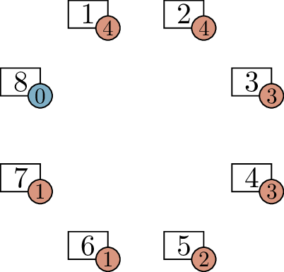
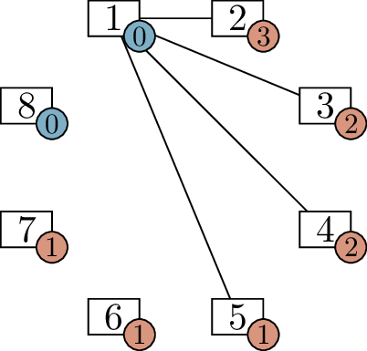
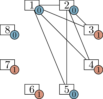
The initial problemStep 1Step 2
Step 3Step 4
Finding a graph with degree sequence \(4, 4, 3, 3, 2, 1, 1, 0\)
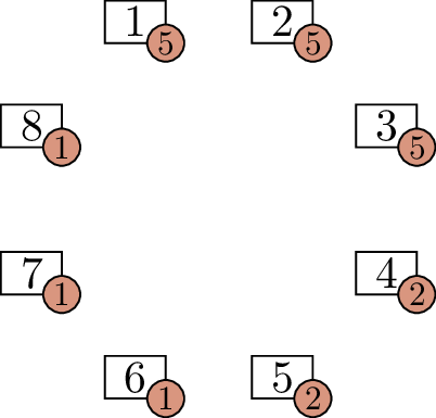
We begin with a graph with no edges in which the demand of each
vertex is equal to the degree we want it to have, as shown in Figure 6.2(a). (Vertex \(8\) starts out inactive; it does not affect
the problem in any way.)
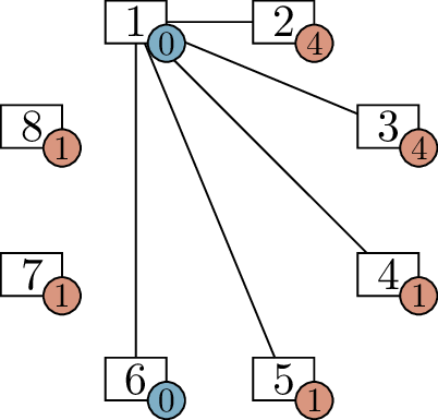
We begin one of the vertices with demand \(4\) (I choose \(1\), though it is also possible to choose
\(2\)) and add edges to the \(4\) other vertices with the highest demands
(vertices \(2\), \(3\), \(4\), and \(5\)). The result is Figure 6.2(b), with one fewer active
vertex.
Our next choice is unique: vertex \(2\), with demand \(3\). The vertices that will become its
remaining neighbors must include vertices \(3\) and \(4\) (with demand \(2\)), as well as one of the vertices with
demand \(1\); we arbitrarily choose it
to be vertex \(5\). Adding the edges
between these vertices and decreasing demand accordingly, we obtain
Figure 6.2(c).
Here, all four remaining vertices are tied for highest demand: their
demands are all \(1\). Our next step
will be to draw an edge between two of its vertices, and any of the ways
to do that are fine. In Figure 6.2(d), we add edge \(36\), leaving only two active vertices, and
in Figure 6.2(e), we add edge \(47\) and finish the problem. We can check
our answer by checking that the label on each vertex in Figure 6.2(a) is equal to the degree
it has in Figure 6.2(e).
In this example, the sequence we started with was graphic; let’s
consider an example where the sequence we start with is not graphic. I
will use the sequence \(5, 5, 5, 2, 2, 1, 1,
1\).
The initial problemStep 1Step 2
Trying to find a graph with degree sequence \(5, 5, 5, 2, 2, 1, 1, 1\)
The first step, going from Figure 6.3(a) to Figure 6.3(b), is completely normal.
We pick vertex \(1\) (we could also
have picked vertex \(2\) or \(3\), since all of them have demand \(5\)) and join it to vertices \(2\) through \(6\) (the \(5\) vertices with the highest demands).
Vertices \(1\) and \(6\) become inactive at this step.
Next, we pick one of the vertices with demand \(4\): say, vertex \(2\). We draw \(4\) edges, one of which must go to \(3\), and the rest must go to vertices with
demand \(1\). There are several ways to
draw the edges, but all of them have a similar result to what is shown
in Figure 6.3(c). Almost all of the
vertices have become inactive.
We can no longer proceed! In Figure 6.3(c), vertex \(3\) has demand \(3\), but we do not have \(3\) other active vertices to connect to. So
we declare that the sequence \(5, 5, 5, 2, 2,
1, 1, 1\) is not graphic, and give up.
Now, where in this process do we need additional proof?
Nothing more is needed with the first example. In principle, once we
have a graph with the right degree sequence, we don’t care if we got it
by a valid algorithm, or an invalid algorithm, or if it came to us in a
dream: we have the answer, and we can check it! But we are in even
better shape than that: we’ve already shown that if the graphic sequence
algorithm produces a graph, then the graph it produces is guaranteed to
have the right degree sequence.
The second example is iffier. A critic might complain that what we’re
doing is similar to taking a crossword, writing in a few random words
without looking at the clues, then pointing to one of the crossing
entries and saying, “There’s no word with the letters Q, X, blank, O. So
there must be a mistake in the crossword.” Sure, there could be a
mistake. But maybe we just made the wrong guesses?
For the specific degree sequence \(5, 5, 5,
2, 2, 1, 1, 1\), we could backtrack and see that if we had made
different choices, we’d be equally stuck. However, we don’t want a
backtracking algorithm; for a longer degree sequence, that would be too
tedious. What we want is an argument that justifies the specific choices
our algorithm makes.
But what is it that we want? We don’t need to prove that a graph with
such a degree sequence must have the edges that we guessed. There could
be multiple solutions, after all! What we need to prove is that whenever
solutions exist, our guess doesn’t eliminate them all: that at least one
of the solutions has the structure that the graphic sequence algorithm
expects.
The Havel–Hakimi theorem
The result we need to prove is known as the Havel–Hakimi theorem:
named after Václav Havel, who proved it in 1955 [52], and S. L. Hakimi, who rediscovered the
corresponding algorithm for testing if a sequence is graphic
in 1962 [46]. Before we
prove it, we will restate it in a different way, closer to how it was
presented by Havel.
Theorem 6.2 (Havel–Hakimi theorem). Let \(G\) be a graph with vertex set \(V(G) = \{1, 2, \dots, n\}\) such that \(\deg(1) \ge \deg(2) \ge \dots \ge
\deg(n)\). Let \(k = \deg(1)\)
and let \(S = \{2, 3, \dots,
k+1\}\).
Then there is a graph \(H\) with
\(V(G) = V(H)\) and with \(\deg_G(x) = \deg_H(x)\) for all \(x\) such that the neighbors of vertex \(1\) in \(H\) are precisely the vertices of \(S\).
How does the Havel–Hakimi theorem justify
the correctness of our algorithm?
In the first step, vertex \(1\) (up to tiebreaks) is exactly the vertex
we will process, and the edges from \(1\) to \(S\) are exactly the edges we add. The
Havel–Hakimi theorem tells us that if there are any graphs \(G\) with the degree sequence we want, then
in particular there is a graph \(H\) in
which the choices we made are correct.
That only applies to the first step—what
about future steps?
In our algorithm, there are never any
edges between two active vertices. So if we only consider the subgraph
induced by the active vertices (with the leftover demands), then every
step is exactly like the first.
The advantage of stating the Havel–Hakimi theorem the way we did is
that it describes a transformation: we want to take graph \(G\) and transform it into another graph
\(H\), without changing the vertices or
their degrees, so that \(H\) has the
edges we want. We’ll do the transformation step by step, so we need a
way to make a minor change to a graph without changing its degree
sequence.
This minor change is an operation called an edge swap. To
perform one in a graph \(G\), we first
find four vertices \(vw\) and \(xy\) such that \(vw\) and \(xy\) are edges of \(G\), but \(vx\) and \(wy\) are not. Then, we delete the edges
\(vw\) and \(xy\) that did exist, and replace them by
the edges \(vx\) and \(wy\) that previously did not exist.
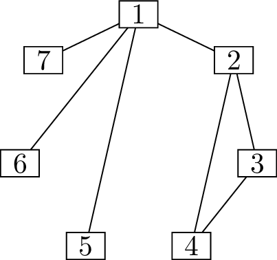
Figure 6.4 shows an example of an edge
swap. You can see how the affected vertices \(v\), \(w\), \(x\), and \(y\) each lose an edge and gain another
edge; thus, the overall degree sequence does not change.
The initial graphSwap edges \(12\) and
\(54\)……for edges \(15\) and \(24\).
An example of an edge swap
We begin by proving a lemma that essentially says, “we can always use
edge swaps to make progress toward what we want.” (I have sneakily
reduced the number of hypotheses, eliminating ones we don’t really need.
vertex \(x\) in Lemma 6.3 is vertex \(1\) in the Havel–Hakimi theorem, which has
the highest degree in \(G\), but we
will not to assume this.)
Lemma 6.3. Let \(x\) be a vertex in a graph \(G\) and let \(S\) be a set of at most \(\deg(x)\) vertices in \(G\) not equal to \(x\) with the highest degrees, breaking ties
arbitrarily.
If not all vertices of \(S\) are
adjacent to \(x\), then we can perform
an edge swap in \(G\) to increase the
number of vertices in \(S\) adjacent to
\(x\).
Proof. Let \(y \in S\) be a
vertex not adjacent to \(x\). Since
\(\deg(x) \ge |S|\), but \(x\) is not adjacent to every vertex in
\(S\), it must also have neighbors
outside \(S\); call one such neighbor
\(z\). To summarize, \(xy\) is not an edge of \(G\), but we wish it were; \(xz\) is an edge of \(G\), but we don’t want it.
We want to fix this state of affairs with an edge swap, but that
needs a fourth vertex.
What kind of fourth vertex \(w\) lets us perform an edge swap that
delete edge \(xz\) and add edge \(xy\)?
At the same time, we must also delete edge
\(yw\) and add edge \(zw\). So \(w\) must be adjacent to \(y\), but not to \(z\).
(It does not matter whether \(w \in
S\) or not, and it does not matter whether \(w\) is adjacent to \(x\) or not.)
This is where our choice of \(S\)
becomes important. We chose the vertices of \(S\) to have the highest degrees. Even if we
broke some ties to do it, we know that the degree of every vertex
in \(S\) is greater than or equal to
the degree of every vertex not in \(S\), other than \(x\). In particular, \(\deg(y) \ge \deg(z)\).
On the other hand, we already have an example of a vertex adjacent to
\(z\), but not \(y\): vertex \(x\). Before we look at any other vertices,
\(z\) is in the lead. To reach \(\deg(y) \ge \deg(z)\), \(y\) must counter that lead at some point:
it must have a neighbor \(z\) does not.
Such a neighbor is exactly the vertex \(w\) we wanted.
By performing the edge swap which deletes edges \(xz\) and \(yw\) and adds edges \(xy\) and \(zw\), We achieve the result we want: \(x\) is adjacent to one more vertex of \(S\). ◻
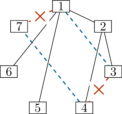
\(x\) has one edge to \(S\)First edge swap
Second edge swapFinal result
Two iterations of Lemma 6.3 in an
example; \(x=1\) and \(S = \{2,3,4\}\)
Figure 6.5 shows two examples of
using the edge swap given by Lemma 6.3.
Throughout, we want vertex \(x=1\) to
become adjacent to all three vertices of \(S =
\{2,3,4\}\). (In fact, \(\deg(x)=4\), which is bigger than \(|S|\). In the proof of the Havel–Hakimi
theorem, we apply Lemma 6.3 to a
case where \(\deg(x) = |S|\), but only
the inequality \(\deg(x) \ge |S|\) is
necessary.)
In Figure 6.5(a), \(x\) has only one neighbor in \(S\): vertex \(2\). We take \(y=3\) (a neighbor \(x\) wants to have in \(S\), but doesn’t) and \(z = 7\) (a neighbor \(x\) has, but doesn’t want). We look for a
third vertex adjacent to \(y\), but not
\(z\), and find vertex \(w=4\) (vertex \(2\) would also have worked). Then, we swap
edges \(17\) and \(34\) for edges \(13\) and \(47\), as shown in Figure 6.5(b).
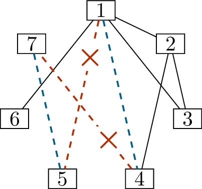
After we do this, \(x\) only has
two neighbors in \(S\): vertices \(2\) and \(3\). It is still not adjacent to vertex
\(4\), so we take \(y=4\); we take \(z=5\) to be the neighbor that \(x\) is going to lose. The two vertices
adjacent to \(y=4\) but not \(z=5\) are \(2\) and \(7\); let’s take \(w=7\). Then, we swap edges \(15\) and \(47\) for edges \(14\) and \(57\), as shown in Figure 6.5(c).
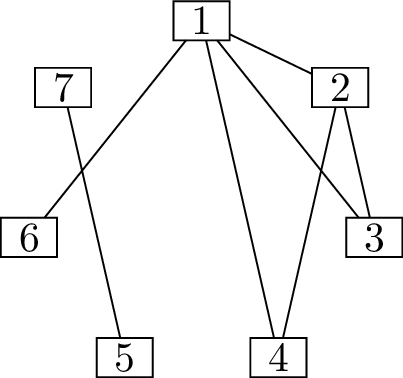
In the final result, shown in Figure 6.5(d),
\(x\) is adjacent to every vertex of
\(S\).
I put Lemma 6.3 first because from here, the proof
of the Havel–Hakimi theorem is essentially just an application of the
lemma, together with the extremal principle. It is a good exercise to
try to do this yourself before reading ahead.
Proof of Theorem 6.2. Of all graphs with the
same vertex set and vertex degrees as \(G\), let \(H\) be chosen to maximize the number of
neighbors of \(1\) in \(S\).
Then actually, all vertices of \(S\)
must be adjacent to \(1\). If not, we
could use Lemma 6.3 (taking \(x=1\)) to increase the number of neighbors
of \(1\) in \(S\). But \(H\) was chosen to have the largest possible
number of such neighbors, so this can’t happen.
Therefore \(H\) is exactly the graph
needed to prove the theorem. ◻
I should say that the graphic sequence algorithm we’ve described is
also known as the Havel–Hakimi algorithm, but it is commonly described
in a different way that I consider less intuitive. Instead of putting
the demands on the vertices and drawing edges, we can think of the
algorithm as modifying a sequence \(d_1 \ge
d_2 \ge \dots \ge d_n\) of the intended degrees. If \(k = d_1\), the highest degree, then the
algorithm places edges from the first vertex to the \(k\) vertices after it. This corresponds to
an operation on sequences, turning \(d_1, d_2,
\dots, d_n\) into \[\underbrace{d_2-1,
d_3 -1, \dots, d_{k+1}-1}_{k \text{ terms}}, d_{k+2}, \dots,
d_n.\] Repeating this operation eventually produces a sequence of
all \(0\)’s (in which case the original
sequence is graphic) or a sequence which is clearly not graphic (for
example, because it contains negative numbers).
More on degree sequences
We only used edge swaps in the proof of the Havel–Hakimi theorem, but
they have other applications. To begin with, we can show the following
theorem:
Theorem 6.4. If two graphs \(G\) and \(H\) have the same vertex set \(V\), and \(\deg_G(x) = \deg_H(x)\) for all \(x \in V\), then we can turn \(G\) into \(H\) by doing edge swaps.
Proof. We prove this by induction on the size of \(V\) (the common vertex set of \(G\) and \(H\)).
When \(|V|=1\), there is nothing to
show: there is only one possible graph on \(1\) vertex.
Assume this is possible for all pairs of \((n-1)\)-vertex graphs, and let \(G\) and \(H\) both have \(n\) vertices. Let \(x\) be a vertex with the highest degree (in
both \(G\) and \(H\)) and let \(S\) be the \(\deg(x)\) vertices with the highest degrees
after \(x\).
By applying Lemma 6.3 repeatedly, we can perform edge
swaps on \(G\) to get a graph \(G'\) in which \(x\)’s neighbors are the vertices in \(S\). We can do the same to \(H\), getting a graph \(H'\) (and so there is also a sequence
of edge swaps that turn \(H'\) into
\(H\), by reversing those edge
swaps).
By induction, there is a sequence of edge swaps that turns \(G' - x\) into \(H' - x\) (both \((n-1)\)-vertex graphs on the same vertex
set). We can perform these edge swaps on \(G'\) instead, and they will work
equally well, turning \(G'\) into
\(H'\). Finally, we know that we
can turn \(H'\) into \(H\).
This shows that we can turn \(G\)
into \(H\), and so by induction, this
works when \(G\) and \(H\) have any number of vertices. ◻
Why is this theorem useful? Well, we know how to answer two possible
questions about potential degree sequences…
Is this sequence graphic? (Is it the degree sequence of a
graph?)
How is this sequence graphic? (Find a graph with this degree
sequence.)
…but there is a third, harder question we can ask:
What is a typical graph with this degree sequence?
That’s deliberately vague. However, Theorem 6.4 is the
beginning of a possible answer to the last question.
What we can do is start with an arbitrary graph which has that degree
sequence, then perform many edge swaps at random, getting a random graph
with this degree sequence.2 We can approximately
answer questions like “are most graphs with this degree sequence
connected” or “what is the average diameter of a graph with this degree
sequence” by sampling many random graphs and analyzing the set of
results.
We can even approximately answer questions like “how many different
graphs have this degree sequence?” To do this, just sample lots of
graphs, then count how many repeats you get. Compare this to how many
repeats you’d expect, if there were \(N\) possible graphs total. This should let
you estimate the most likely value of \(N\).
There is one difficulty to the procedure I’m outlining to you so
cheerfully and optimistically, and that is the requirement of performing
“many” edge swaps. Obviously, just one or two random edge swaps are not
enough: the result is guaranteed to be very similar to our non-random
starting graph. As the number of edge swaps grows, the dependence on the
starting graph slowly decreases. However, it’s still not known in
general how many edge swaps are necessary to make that dependence
negligible. Without that knowledge, the random sampling algorithm cannot
be considered reliable.
Practice problems
Using the degree sequence algorithm, or in some other way,
determine which of the sequences below are graphic:
\(7, 6, 5, 4, 3, 2,
1\).
\(4, 4, 3, 3, 3, 2,
2\).
\(6, 6, 5, 3, 2, 2, 1,
1\).
\(n, n, n, \underbrace{3, 3, \dots,
3}_{n \text{ times}}\) (for any \(n\)).
For the sequences that are graphic, construct graphs with those
degree sequences.
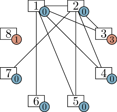
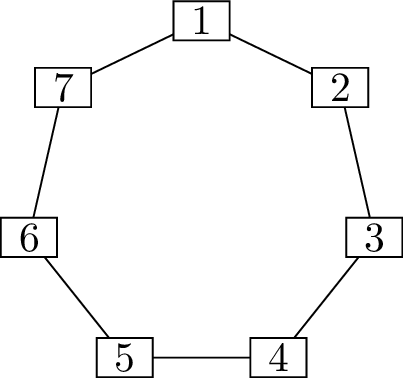
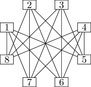
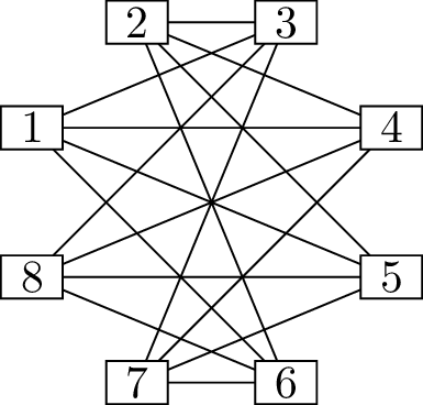
Let \(G\) be the graph on the
left in the diagram below, and let \(H\) be the graph on the right.
Corresponding vertices have the same degrees, and the two graphs are
isomorphic, but they are not the same graph: they have different edges.
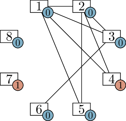
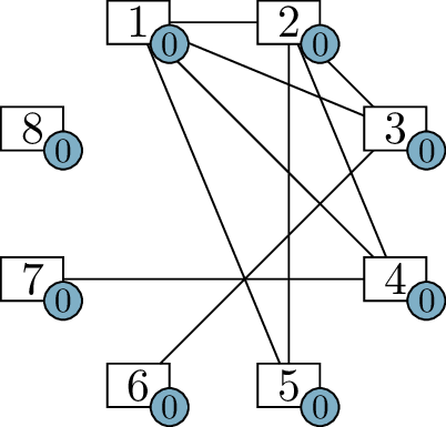
\(G\) has all edges between \(\{1,2,3,4\}\) and \(\{5,6,7,8\}\), while \(H\) has all edges between \(\{1,2,5,6\}\) and \(\{3,4,7,8\}\).
Find a sequence of edge swaps to turn \(G\) into \(H\). (Four edge swaps are enough.)
Let me tell you another story.
The other day, I was at another very large party. Once again, each
person at the party knew a different number of people, with one
exception: I personally knew the same number of people as another guest,
named Pasha. In addition, I can promise you that everyone at this party
knew at least one other person.
The surprising thing is this: I did not know Pasha! How could this
happen, and why does this not contradict Proposition 6.1?
In Problem 6.1, I included the
condition that everyone at the party knew at least one other person. If
this condition is dropped, then there is another possible graph: how can
we find it? (What should its degree sequence be?)
There are \(7\) possible graphs
with the vertex set \(\{1, 2, 3, 4,
5\}\) such that \(\deg(1) = \deg(2) =
3\) and \(\deg(3) = \deg(4) = \deg(5) =
2\). Find all of them, and demonstrate directly that we can turn
any one of them into any other via edge swaps.
There is another proof of Theorem 6.4 that is
closer to our argument for the Havel–Hakimi theorem.
Specifically, if \(G\) and \(H\) have the same vertex set, and every
vertex has the same degree in \(G\) and
in \(H\), then we can measure “how far
away” \(G\) and \(H\) are from each other by asking: how many
edges does \(G\) have that are not also
edges of \(H\)? Now we can do the
following:
Prove that if \(G\) and \(H\) are not literally the same graph, then
there is an edge swap we can perform on \(G\) to reduce “how far away” it is from
\(H\).
Under what conditions on \(a\),
\(b\), and \(n\) is a sequence of the form \[\underbrace{a, a, \dots, a}_n, \underbrace{b, b,
\dots, b}_n\] a graphic sequence?
Let \(G\) be an \(n\)-vertex graph whose vertices \(1, 2, \dots, n\) have degrees \(d_1, d_2, \dots, d_n\) respectively, sorted
in descending order: \[d_1 \ge d_2 \ge \dots
\ge d_n.\] Then \(d_1\) (the
maximum degree of \(G\)) can be at most
\(n-1\); in fact, it can be at most the
number of nonzero degrees among \(d_2, \dots,
d_n\).
Explain why this is equivalent to the following inequality: \[d_1 \le \sum_{i=2}^n \min\{d_i, 1\}.\]
Here, \(\min\{a,b\}\) is simply the
smaller of the two numbers \(a\) and
\(b\).
Prove the following inequality, which is a \(2\)-vertex generalization of the previous
one: \[d_1 + d_2 \le 2 + \sum_{i=3}^n
\min\{d_i, 2\}.\] (Consider the number of edges between vertices
\(1\) and \(2\) and the rest of the graph. Why is the
“\(2+\)” there?)
In general, we have an inequality of the form \[\sum_{i=1}^k d_i \le f(k) + \sum_{j=k+1}^n
\min\{d_j, k\}\] for each \(k \in
\{1,\dots,n\}\). What is the best possible function \(f(k)\) that makes this inequality true? (I
ask for “best possible” because some incredibly big function like \(f(k) = 2^{2^{2^k}}\) will also work, but
will not be as useful as the smallest possible number you could put
there.)
More is true: a theorem of Pál Erdős and Tibor Gallai [30] states that if a sequence
\(d_1, d_2, \dots, d_n\) satisfies the
inequality in part (c) for every \(k\),
and the sum \(d_1 + d_2 + \dots + d_n\)
is even, then the sequence is graphic. This is an alternative way to
check whether a sequence is graphic.
Footnotes
This appears to be a very common story to tell. In
West’s Introduction to Graph Theory[104], a version of it appears as “The Handshake
Problem”, and another version was a problem in the 1985 British
Mathematical Olympiad.↩︎
Fine print: this does not sample a graph uniformly at
random. Essentially, it samples a graph with probability proportional to
how many edge swaps are possible to do in it. But that’s a known bias we
can account for.↩︎