The definition of a graph isomorphism is sufficiently fundamental
that no self-respecting graph theory book could skip it. Most authors
wouldn’t put this chapter so close to the beginning of the book,
though.
The reason I wanted to introduce isomorphic graphs early on is for
the sake of the isomorphism game in Section 2.3. By playing this game,
you can discover concepts like vertex degree, subgraphs, connected
components, and others naturally: that is, you come up with them because
you need them for something. Later chapters will tell you the full story
of these concepts, and I will then try to motivate them by telling you
what they’re good for—but another answer to what they’re all good for is
to act as graph invariants.
I begin with the definition of circulant graphs for several reasons.
They will be useful to us many times later on, because they’re a very
flexible family of graphs. Their definition is also good to understand
now: it will give you some practice with modular arithmetic, which will
help us with other constructions in graph theory that have rotational
symmetry. Finally, they give some good examples of “unexpected” graph
isomorphisms, as in Proposition 2.1, and in exercises at
the end of this chapter.
Circulant graphs
I have a surprising question to ask you, but before I do, I want to
tell you about a family of graphs: the circulant graphs. (A set of
graphs is called a “family” for the same reason that a set of people is
called a family: when they’re all related. But the relationship between
graphs in a family is more abstract and metaphorical: they are graphs
that all share an important property, or that are all defined in similar
ways.)
To pick out a specific circulant graph, we need two pieces of
information: an integer \(n\) (which
will just be the number of vertices) and a set \(\{d_1, d_2, \dots, d_k\}\) of offsets, or
jumps: integers between \(1\) and \(n/2\). Once we have this information, the
informal way to define the circulant graph is as follows: we put \(n\) vertices in a circle, and join two
vertices by an edge if they are \(d_i\)
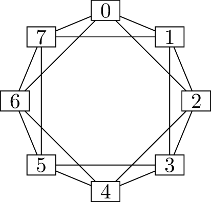
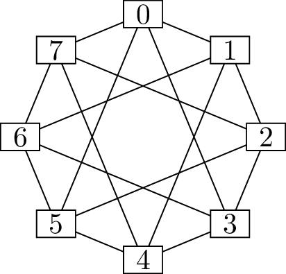
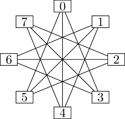
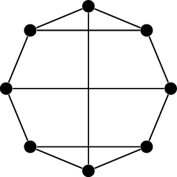
steps apart in the circle, for some \(i\). For example, Figure 2.1(a) shows a circulant graph with
\(n=8\) vertices and with the set of
jumps \(\{1,2\}\): two vertices are
adjacent if they are next to each other around the circle, or two steps
apart.
This is only an informal definition because we prefer not to define
graphs in terms of how they’re drawn: it’s not forbidden to do so, but
it’s discouraged, because we don’t want to get attached to one specific
way of drawing the graph. After all, a graph is not the drawing: it is
just a set of vertices and edges.
The mathematically precise way to describe the rules that define a
circulant graph is with modular arithmetic. If you are already familiar
with it, feel free to skip ahead to Definition 2.2. We will need to use
modular arithmetic several times throughout this book, so let me
introduce it now in a bit more detail than we need just to understand
circulant graphs.
The fundamental notion of modular arithmetic is congruence modulo
\(n\), defined as follows:
Definition 2.1. Two integers \(a\) and \(b\) are congruent modulo a
positive integer \(n\) when \(a\) and \(b\) differ by a multiple of \(n\): \(a-b =
kn\) for some \(k\). We write
this \(a \equiv b \pmod n\).
For all \(n\ge 1\), every
integer \(a\) is congruent to exactly
one element of the set \(\{0,1,\dots,n-1\}\) modulo \(n\); we refer to that element of \(\{0,1,\dots,n-1\}\) as \(a\) modulo \(n\), written \(a \bmod n\).
Modular arithmetic is used in situations where numbers “wrap around
to the start” after \(n\), so that
\(n+1\) is the same as \(1\), and \(n+2\) is the same as \(2\), and so on. A common real-life
situation of this type is clock arithmetic: the hours are labeled \(1\) through \(12\), but the hour after \(12\) is \(1\), not \(13\). The hours on a clock are placed in a
circle, just as the vertices of a circulant graph, and we’re going to
use modular arithmetic for the same purpose!
You can treat the statement \(a \equiv b
\pmod n\) as being a relaxed kind of equality. Like equality, you
can often apply the same operation to both sides to get another true
statement:
\(3 \equiv 13 \pmod{10}\), so
\(3+4 \equiv 13+4 \pmod{10}\), or \(7 \equiv 17 \pmod{10}\).
\(4 \equiv 52 \pmod{24}\), so
\(4 \cdot 5 \equiv 52 \cdot 5
\pmod{24}\), or \(20 \equiv 260
\pmod{24}\).
\(6 \equiv -1 \pmod{7}\), so
\(6^2 \equiv (-1)^2 \pmod 7\), or \(36 \equiv 1 \pmod{7}\).
The one common operation you must be careful about is division. It is
not always okay to go from \(a \equiv b \pmod
n\) to \(\frac ac \equiv \frac bc \pmod
n\). This is only allowed if \(c\) and \(n\) have no divisors in common! For
example, we can divide both sides of \(6
\equiv 36 \pmod{10}\) by \(3\)
to get \(2 \equiv 12 \pmod{10}\): a
true statement. But if we divided both sides by \(2\), we’d get \(3
\equiv 18 \pmod{10}\), which is false! (A quick way to see this:
two positive integers are congruent modulo \(10\) if and only if their last digits are
the same.)
There is much more to learn about modular arithmetic, but we’ve seen
enough to get us through this book. So let’s finally state the formal
definition of a circulant graph:
Definition 2.2. For any \(n\ge 1\) and any set of integers \(\{d_1, d_2, \dots, d_k\}\) all between
\(1\) and \(n/2\), the circulant graph \(\operatorname{Ci}_n(d_1, d_2, \dots,
d_k)\) is the graph with vertex set \(\{0,1,\dots,n-1\}\) in which two vertices
\(x,y\) are adjacent whenever \(x-y \equiv \pm d_i \pmod n\) for some \(i\).
Looking back at Figure 2.1,
you should check that this definition matches what you see in the
diagrams, and that it matches what you’d expect from the informal
definition.
Why do we say that \(d_1, d_2, \dots, d_k\) must be between
\(1\) and \(n/2\)?
Larger offsets would not mess up the
definition, but they’re unnecessary. If we had an offset \(d_i\) bigger than \(n\), we could replace it by the
offset \(d_i \bmod n\). If we had an
offset \(d_i\) between \(n/2\) and \(n\), we could replace it by \(n - d_i\).
Are these the same?
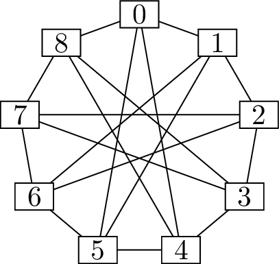
The surprising question that I want to ask you now is this: are the
graphs \(\operatorname{Ci}_9(1,2)\) and
\(\operatorname{Ci}_9(1,4)\) the same?
Before you answer, “No, obviously not,” let me make my case.
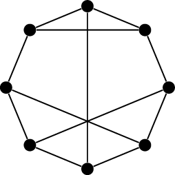
Comparing \(\operatorname{Ci}_9(1,2)\) to \(\operatorname{Ci}_9(1,4)\)
In Figure 2.2, the first two
diagrams are just the standard diagrams of \(\operatorname{Ci}_9(1,2)\) and \(\operatorname{Ci}_9(1,4)\). However,
Figure 2.2(c) is something slightly
different: it is also a diagram of \(\operatorname{Ci}_9(1,4)\), but it has the
same “shape”—the edges are drawn in all the same places—as Figure 2.2(a), which shows \(\operatorname{Ci}_9(1,2)\).
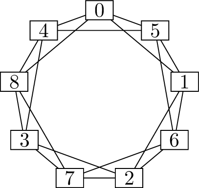
How do we know Figure 2.2(c) is also a diagram of
\(\operatorname{Ci}_9(1,4)\)?
For each vertex, you can check that its
neighbors are the same in both Figure 2.2(b)
and Figure 2.2(c). For example, the
neighbors of vertex \(1\) are vertices
\(0\), \(2\), \(5\), and \(6\) in both diagrams.
I can’t argue with the definitions, though: \(\operatorname{Ci}_9(1,2)\) and \(\operatorname{Ci}_9(1,4)\) are not the same
graph, because they have a different set of edges. For example, \(\{0,2\} \in E(\operatorname{Ci}_9(1,2))\)
but \(\{0,2\} \notin
E(\operatorname{Ci}_9(1,4))\). And yet, Figure 2.2(a) and Figure 2.2(c) show us that the two
graphs are almost identical: you can turn one into the other just by
renaming the vertices! If you think about the sort of questions we asked
in Chapter 1—for example, the largest
number of vertices we can select that are all adjacent—it’s clear that
any answer we find in \(\operatorname{Ci}_9(1,2)\) will also work
in \(\operatorname{Ci}_9(1,4)\), and
vice versa.
In \(\operatorname{Ci}_9(1,4)\), the vertices
\(1\), \(5\), and \(6\) form a triangle: the edges \(15\), \(16\), and \(56\) are all present. Does this correspond
in any way to a triangle in \(\operatorname{Ci}_9(1,2)\)?
Yes, but we have to do some “translation”.
Vertices \(1\), \(5\), and \(6\) are in the same place in Figure 2.2(c) as vertices \(2\), \(1\), and \(3\) in Figure 2.2(a),
so vertices \(2\), \(1\), and \(3\) form a triangle in \(\operatorname{Ci}_9(1,2)\).
When this relationship exists between two graphs \(G\) and \(H\)—when we can turn \(G\) into \(H\) by just changing the names of the
vertices—we say that \(G\) and \(H\) are isomorphic. For small graphs, this
is often easy to show with a diagram, as in Figure 2.2, but it would be
difficult both to draw and to check if the graphs were larger. If we had
to describe how \(\operatorname{Ci}_9(1,2)\) and \(\operatorname{Ci}_9(1,4)\) correspond to
each other without drawing the diagram, we’d want to make a list of the
way we rename the vertices. For example, to turn Figure 2.2(c) into Figure 2.2(a), we rename vertex \(1\) to \(2\), vertex \(2\) to \(4\), vertex \(3\) to \(6\), and so on. The mathematical object
that describes such a correspondence is a function: a function \(\varphi \{0,1,\dots,8\} \to
\{0,1,\dots,8\}\). In general, \(\varphi\) should be a function from \(V(G)\) to \(V(H)\). Not just any function will do,
however:
Definition 2.3. An isomorphism
from a graph \(G\) to a graph \(H\) is a function \(\varphi\colon V(G) \to V(H)\) that
satisfies the following properties:
\(\varphi\) is a bijection:
for every vertex \(y \in V(H)\) there
should be a vertex \(x \in V(G)\) such
that \(\varphi(x) = y\). In other
words, \(\varphi\) should have an
inverse \(\varphi^{-1} \colon V(H) \to
V(G)\).
This makes the function a true correspondence, pairing each
vertex in one graph with a vertex in the other.
\(\varphi\) preserves the
edges: for every two vertices \(x, y \in
V(G)\), we have the equivalence \[xy
\in E(G) \iff \varphi(x) \varphi(y) \in E(H).\] In other words,
applying the function \(\varphi\) to go
from \(G\) to \(H\) does not change which vertices are
adjacent to each other.
When there is an isomorphism from \(G\) to \(H\), the graphs \(G\) and \(H\) are isomorphic to each
other.
You should not be surprised by the two properties we asked for in
this definition. If you think about the things you’d do to check if the
diagrams in Figure 2.2(a)
and Figure 2.2(c) are the same, the two
properties are just formally describing what you’d do. First, you’d
check that for every vertex in one diagram, there’s a vertex in the same
place in the other diagram (verifying that \(\varphi\) is defined for all inputs, and
that it’s a bijection). Second, you’d want to check that every edge
drawn in one diagram is also present in the other diagram (verifying
that \(\varphi\) preserves the
edges.)
Figure 2.2 suggests a particular
isomorphism \(\varphi\), given by the
following table: \[\begin{array}{r|ccccccccc}
\text{vertex of }\operatorname{Ci}_9(1,4) & 0 & 1 & 2 &
3 & 4 & 5 & 6 & 7 & 8\\
\hline
\varphi(\text{vertex}) & 0 & 2 & 4 & 6 & 8 & 1
& 3 & 5 & 7
\end{array}\] This is one possible concise way to specify an
isomorphism, although for small graphs, a diagram like in Figure 2.2 is just as good. You
should think of \(\varphi\) as being
like a dictionary that translates from names in \(\operatorname{Ci}_9(1,4)\) to names in
\(\operatorname{Ci}_9(1,2)\). In the
“language” of \(\operatorname{Ci}_9(1,4)\), the statement
“\(1\) is adjacent to \(2\), but not to \(3\)” is true. That’s a false statement
about \(\operatorname{Ci}_9(1,2)\), but
it becomes a true one after it’s been “translated”! When translated, it
becomes “\(\varphi(1)\) is adjacent to
\(\varphi(2)\), but not to \(\varphi(3)\)”, or “\(2\) is adjacent to \(4\), but not to \(6\)”.
(Just as with foreign languages, such a dictionary can have cognates:
vertices like \(0\) that have the same
role in both graphs. It can also have false cognates: both graphs have a
vertex \(1\), but \(\operatorname{Ci}_9(1,2)\)’s vertex \(1\) does not correspond to \(\operatorname{Ci}_9(1,4)\)’s vertex \(1\).)
In practice, the best reason to work with the function \(\varphi\) formally is in a proof: if you
have two graphs of arbitrary size given by abstract rules, and you want
to prove they’re isomorphic, then you can’t draw a diagram—you have to
give an isomorphism and verify that it works. Here’s an example of such
a proof:
Proposition 2.1. For all odd integers \(n\), the graph \(\operatorname{Ci}_n(1,\frac{n-1}{2})\) is
isomorphic to \(\operatorname{Ci}_n(1,2)\).
Proof. Modular arithmetic gave us the formal definition of
the circulant graphs, and it can also give us the isomorphism! To find
it, we need to find a pattern in the \(n=9\) case (where we already have an
isomorphism) and generalize.
Is there a pattern in the table defining
the isomorphism \(\varphi\) from \(\operatorname{Ci}_9(1,4)\) to \(\operatorname{Ci}_9(1,2)\)?
Yes; probably the first one you will spot
is that the values of \(\varphi\) in
the table begin by going up by \(2\)’s
from left to right.
In fact, we can check that the formula \(\varphi(x) = 2x \bmod 9\) works for every
value in the table, and so to prove the generalization we want, we can
try defining \(\varphi(x) = 2x \bmod
n\).
To check that \(\varphi\) is a
bijection, we can find an inverse for it. In this case, there happens to
be an inverse with a short formula: \(\varphi^{-1}(x) = \frac{n+1}{2} \cdot x \bmod
n\). We can check that this really is an inverse, because \[\frac{n+1}{2} \cdot 2x = (n+1)x \equiv x \pmod
n.\] When working modulo \(n\),
multiplication by \(\frac{n+1}{2}\)
undoes multiplication by \(2\), and
vice versa. This is usually the best way to proceed: it’s possible to
check that \(\varphi\) is a bijection
by checking that it’s injective and surjective (one-to-one and onto),
but this doesn’t usually save us any work, and the inverse might be
useful for us.
Next, we check that \(\varphi\) maps
vertices adjacent in \(\operatorname{Ci}_9(1,\frac{n-1}{2})\) to
vertices in \(\operatorname{Ci}_9(1,2)\). If two vertices
\(x\) and \(y\) are adjacent in \(\operatorname{Ci}_9(1,4)\), it could be for
four reasons; we could have \(x-y \equiv 1
\pmod n\), or \(x-y \equiv -1 \pmod
n\), or \(x-y \equiv \frac{n-1}{2}
\pmod n\), or \(x-y \equiv
-\frac{n-1}{2} \pmod n\).
If \(x-y \equiv 1 \pmod n\),
then \(\varphi(x) - \varphi(y) = 2(x-y) \equiv
2 \pmod n\).
If \(x-y \equiv -1 \pmod n\),
then \(\varphi(x) - \varphi(y) = 2(x-y) \equiv
-2 \pmod n\).
If \(x-y \equiv \frac{n-1}{2} \pmod
n\), then \(\varphi(x) - \varphi(y) =
2(x-y) \equiv 2(\frac{n-1}{2}) = n-1 \equiv -1 \pmod
n\).
Finally, if \(x-y \equiv -\frac{n-1}{2}
\pmod n\), then \(\varphi(x) -
\varphi(y) = 2(x-y) \equiv 2({-\frac{n-1}{2}})\), which
simplifies to \(1-n\), and \(1-n \equiv 1 \pmod n\).
We have an if-and-only-if statement, so normally the next step would
be to check the converse: either that \(\varphi\) sends non-adjacent vertices in
\(\operatorname{Ci}_n(1,\frac{n-1}{2})\) to
non-adjacent vertices in \(\operatorname{Ci}_n(1,2)\), or that \(\varphi^{-1}\) sends adjacent vertices in
\(\operatorname{Ci}_n(1,2)\) to
adjacent vertices in \(\operatorname{Ci}_n(1,\frac{n-1}{2})\). In
this case, however, we can skip that step by doing some counting
instead.
Both \(\operatorname{Ci}_n(1,\frac{n-1}{2})\) and
\(\operatorname{Ci}_n(1,2)\) both have
\(2n\) edges: each one is a circulant
graph with two offsets, and for each offset \(d_i\), there are \(n\) pairs \(x,y\) such that \(x - y \equiv d_i \pmod{n}\).
Is it always true for circulant graphs
that the number of offsets tells you the number of edges?
Almost always, with one exception: when
\(n\) is even, the offset \(\frac n2\) only produces half the edges
you’d expect. This is because \(x - y \equiv
\frac n2 \pmod n\) and \(x - y \equiv
-\frac n2 \pmod n\) are the same condition! Intuitively, going
\(\frac n2\) steps left around the
circle is the same as going \(\frac
n2\) steps right when \(n\) is
even: both go to the opposite vertex on the circle.
We’ve already checked that \(\varphi\) is a bijection that sends each of
the \(2n\) edges of \(\operatorname{Ci}_n(1,\frac{n-1}{2})\) to
an edge of \(\operatorname{Ci}_n(1,2)\). This “uses up”
all \(2n\) edges of \(\operatorname{Ci}_n(1,2)\). So for a pair
of vertices that are not adjacent in \(\operatorname{Ci}_n(1,\frac{n-1}{2})\),
their images cannot be adjacent in \(\operatorname{Ci}_n(1,2)\), verifying the
converse.
This completes the proof that \(\varphi\) is an isomorphism from \(\operatorname{Ci}_n(1,\frac{n-1}{2})\) to
\(\operatorname{Ci}_n(1,2)\), showing
also that the two graphs are isomorphic. ◻
An isomorphism from \(G\) to \(H\) reveals a way in which \(G\) is the same as \(H\), so an isomorphism from a graph \(G\) to \(G\) itself reveals a way in which \(G\) is the same as \(G\). This doesn’t seem useful at first: we
already know that \(G\) is the same as
\(G\). However, it is useful: it
reveals symmetry in the graph. For example, one of the main reasons
circulant graphs matter in graph theory is their cyclic symmetry:
rotating one of the diagrams in Figure 2.1
by \(45^\circ\), or one of the graphs
in Figure 2.2 by \(40^\circ\), doesn’t change the shape of the
diagram. To state this precisely, we need to discuss automorphisms.
Definition 2.4. An automorphism
of a graph \(G\) is an isomorphism from
\(G\) to itself.
To describe the symmetry of an \(n\)-vertex circulant graph, we might say
that the function \(\alpha\) which
rotates its standard diagram by \(\frac{360^\circ}{n}\) is an
automorphism.
What is the definition of \(\alpha\) using modular arithmetic?
It is the function from \(\{0,1,\dots,n-1\}\) to \(\{0,1,\dots,n-1\}\) given by \(\alpha(x) = x+1 \bmod n\).
We can also spot a different kind of symmetry in the diagrams of our
circulant graphs: if you reflect them, swapping left and right, the
shape does not change. This corresponds to a different isomorphism \(\beta \colon \{0,1,\dots,n-1\} \to
\{0,1,\dots,n-1\}\), where \(\beta(x) =
-x \bmod n\).
Different diagrams can make different automorphisms easier to see,
although the automorphism does not depend on the diagram: \(\alpha\) and \(\beta\) are automorphisms of a circulant
graph directly from the definition, regardless of how we draw it. More
complicated symmetries might not even be possible to illustrate in a
diagram!
Even if a graph \(G\) has no
symmetries to speak of, the function \(\varphi
\colon V(G) \to V(G)\) defined by \(\varphi(x) = x\) for all \(x \in V(G)\) is an automorphism of \(G\). This is called the identity
automorphism or trivial automorphism, and is much less
exciting to discover. (It has a name mostly so that we can talk about
automorphisms other than the trivial one, or about graphs that do or
don’t have nontrivial automorphisms.)
The isomorphism game
How do we find an isomorphism between two graphs when their diagrams
don’t completely line up? And when an isomorphism doesn’t exist, how can
we tell? We don’t want to use brute force: with two \(n\)-vertex graphs, there are \(n!\) possible bijections, which is too many
to check by hand even for fairly small \(n\).
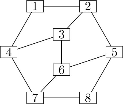
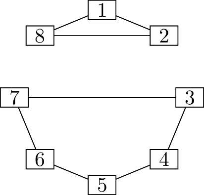
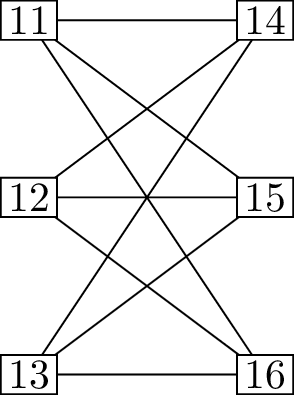
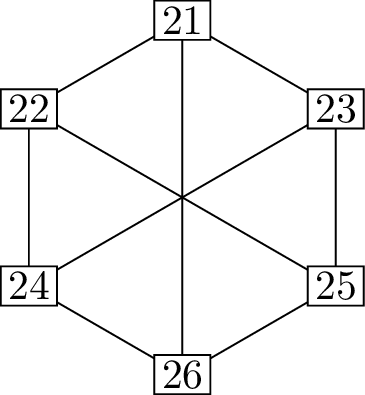
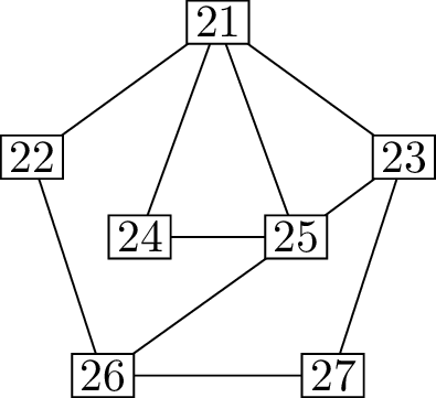
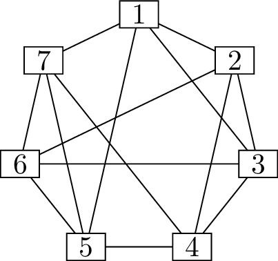
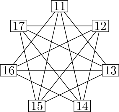
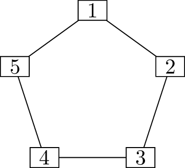
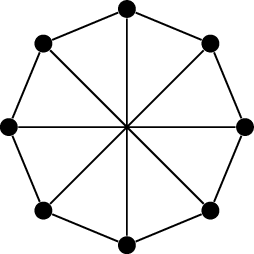
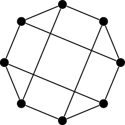
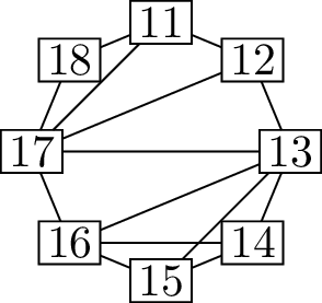
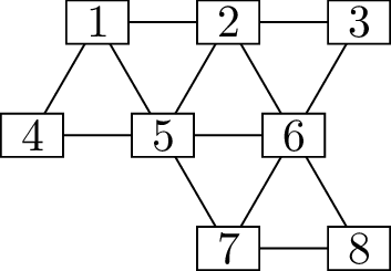
To teach you how to do it, I will teach you to play the “isomorphism
game”. In this game, I show you three graphs. Two of them are isomorphic
to each other, and the third is different. The goal is to identify which
graph is the odd one out, and to find an isomorphism between the other
two. Let me show you how the game is played on an example.
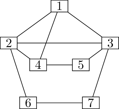
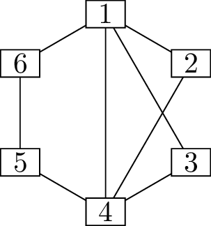
The graph \(G_1\)The graph \(G_2\)The graph \(G_3\)
A three-graph set for the isomorphism game
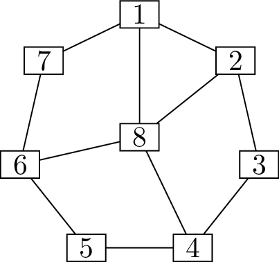
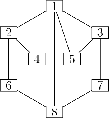
In Figure 2.3, if we consider
the possibility that \(G_1\) and \(G_2\) are isomorphic, how could we begin to
find the isomorphism? A good start is to look for a distinguishing
feature of some of the vertices. Be careful, though! Something like, “In
\(G_1\), vertex \(8\) is all by itself in the middle, unlike
the others, which are arranged in a circle” is not a distinguishing
feature of vertex \(8\)’s role in the
graph, but merely in the diagram; it’s not useful.
We look, instead, for distinguishing features that can’t disappear
when we rearrange the vertices and relabel them. For example, vertex
\(8\) of \(G_1\) has four neighbors: \(1\), \(2\), \(4\), and \(6\). An isomorphism \(\varphi\colon V(G_1) \to V(G_2)\) must
preserve the edges \(18, 28, 48, 68\):
the pairs \(\varphi(1)\varphi(8)\),
\(\varphi(2)\varphi(8)\), \(\varphi(4)\varphi(8)\), and \(\varphi(6)\varphi(8)\) must be edges of
\(G_2\). So \(\varphi(8)\) is a vertex of \(G_2\) with four neighbors: \(\varphi(1)\), \(\varphi(2)\), \(\varphi(4)\), and \(\varphi(8)\). Which vertex can that be? It
can only be vertex \(1\). So we can
deduce that if the isomorphism \(\varphi\) exists, then \(\varphi(8)=1\).
This has given us a foothold, and now we can build on it: to a
complete isomorphism, or to a contradiction. Vertices \(1, 2, 4, 6\) (the neighbors of \(8\)) in \(G_1\) must be sent to vertices \(2, 3, 5, 8\) in \(G_2\): the neighbors of \(1\), which is \(\varphi(8)\). But can we distinguish them
further? Well, in \(G_1\), \(1\) and \(2\) are also adjacent to each other, so
\(\varphi(1)\) and \(\varphi(2)\) must be adjacent. The only
adjacent pair of neighbors that vertex \(1\) has in \(G_2\) is the pair \(\{3,5\}\). So \(\{\varphi(1), \varphi(2)\}\) must be equal
to \(\{3,5\}\), in some order.
We don’t like the words “in some order”—that way lies brute-force
checking of cases. But in this case, there’s an explanation for it. Do
you see that in Figure 2.3(a),
if we draw a straight line passing through vertices \(5\) and \(8\), then it is a line of symmetry of the
diagram? That symmetry gives us an automorphism of \(G_1\), and that automorphism swaps vertices
\(1\) and \(2\). This means that vertices \(1\) and \(2\) play identical roles, as far as
isomorphisms go: anything one of them can do, the other can do just as
well. We can arbitrarily decide \(\varphi(1)=3\) and \(\varphi(2)=5\) without fear of an error.
(See how useful automorphisms can be, after all?)
At this point, the rest of \(\varphi\) can be determined. The neighbors
of \(2\) in \(G_1\) are \(1\), \(3\), and \(8\). The neighbors of \(5 = \varphi(2)\) in \(G_2\) are \(1 =
\varphi(8)\), \(3 =
\varphi(1)\), and \(4\). Two out
of three neighbors have already been matched up by \(\varphi\), so the remaining pair must also
go together: \(\varphi(3) = 4\). Going
around the circle, we can find where \(\varphi\) sends \(4, 5, 6, 7\) and get the following
isomorphism: \[\begin{array}{r|cccccccc}
\text{vertex of }G & 1 & 2 & 3 & 4 & 5 & 6 &
7 & 8 \\
\hline
\varphi(\text{vertex}) & 3 & 5 & 4 & 2 & 6 & 8
& 7 & 1
\end{array}\] We’re halfway done with the game. How do we play
the other half, and explain why \(G_1\)
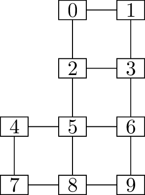
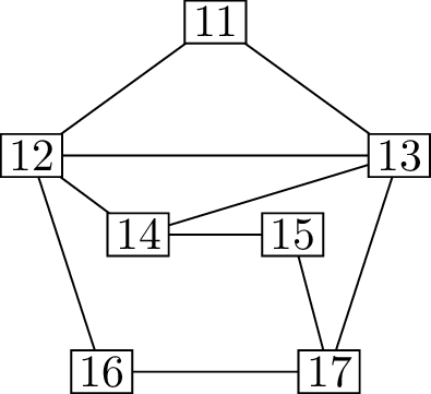
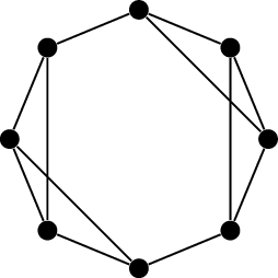
and \(G_3\) are not isomorphic?
The argument begins with the same way; we look for a distinguishing
feature. As before, if \(\psi \colon V(G_1)
\to V(G_3)\) is an isomorphism, then \(\psi(8)\) must be a vertex of \(G_3\) with four neighbors: \(\psi(1)\), \(\psi(2)\), \(\psi(4)\), and \(\psi(8)\). Which vertex can that be? Well,
there is no such vertex! In \(G_3\),
vertices \(1\) and \(8\) have two neighbors, and the rest each
have three neighbors; no vertex has four. So \(\psi\) cannot exist: \(G_1\) and \(G_3\) are not isomorphic.
Is it correct to say that \(G_1\) is not isomorphic to \(G_3\) because vertex \(1\) has three neighbors in \(G_1\), but only two neighbors in \(G_3\)?
No: an isomorphism is allowed to change
which vertex is “vertex \(1\)”.
Is it correct to say that \(G_1\) is not isomorphic to \(G_3\) because \(G_1\) has three vertices (\(3\), \(5\), and \(7\)) with two neighbors each, but \(G_2\) has only two such vertices (\(1\) and \(8\))?
Yes: if there were an isomorphism \(\psi\colon V(G_1) \to V(G_3)\), then \(\psi(3)\), \(\psi(5)\), and \(\psi(7)\) would be three different vertices
with two neighbors each. But there are not three such vertices in \(G_3\).
Is it correct to say that \(G_1\) is isomorphic to \(G_2\) just because for every number \(k\), the two graphs have the same number of
vertices with \(k\) neighbors?
No: we must find the isomorphism before we
draw this conclusion. It’s possible for two graphs to agree in this way,
and yet not be isomorphic, and you’ll see examples of this on the next
page.
In general, to prove that two graphs are not isomorphic, it’s enough
to find any difference between the two graphs that any isomorphism must
preserve: something that’s inherent to the structure of the graph, and
not a feature of the vertex labels or the way the graph is drawn.
Before telling you more about such properties, I will let you
discover some of them for yourself as you play the isomorphism game.
(Try doing this yourself before you look at any spoilers.)
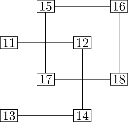
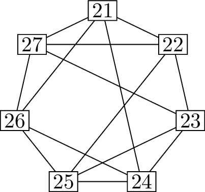
Problem 2.1. Determine which of the three graphs
below is the odd one out, and find an isomorphism between the other
two.
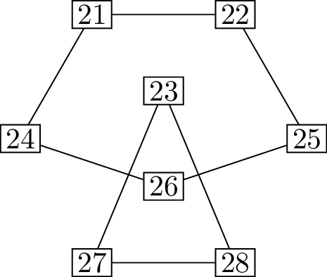
Problem 2.2. Determine which of the three graphs
below is the odd one out, and find an isomorphism between the other
two.
Problem 2.3. Determine which of the three graphs
below is the odd one out, and find an isomorphism between the other
two.
Problem 2.4. Determine which of the three graphs
below is the odd one out, and find an isomorphism between the other
two.
Problem 2.5. Determine which of the three graphs
below is the odd one out, and find an isomorphism between the other
two.
Graph invariants
When playing the isomorphism game, you may say things like, “These
two graphs are not the same as that other graph, because these two
graphs both \(X\), and that other graph
does not \(X\). But a graph that \(X\) can’t be isomorphic to a graph that
does not \(X\).” Whenever you can say
that, \(X\) is called a graph
invariant:
Definition 2.5. A graph
invariant is any property of a graph (a result of any kind that
can be computed from the graph) such that, whenever two graphs \(G\) and \(H\) are isomorphic, they must agree in that
property.
Graph invariants can be binary (true or false), or numerical (like
the number of vertices or edges), or even more complicated, such as a
sequence of numbers. They’re called “invariants” because don’t vary:
they can’t be changed by drawing the diagram differently, or by
relabeling the vertices. In other words, two isomorphic graphs have to
agree on all graph invariants.
Sometimes graph invariants are also called “graph properties”. Using
the word “graph property” is also taking a philosophical stance: it’s
implying that the only true graph properties—the only properties of
graphs that are worth studying in the discipline of graph theory—are
graph invariants! I think this is true, though I will carve one or two
exceptions out for myself in a couple of pages.
Of course, as mathematicians we can’t just intuit our way into
claiming something is a graph invariant: we have to prove it. I will
show you two of these proofs, one for a numerical invariant and one for
a true/false invariant. Lots of these proofs are very similar to each
other, and become boring once you get the hang of them, but I encourage
you to try writing one or two yourself until you get to the point where
you can see how you’d go about writing it before you even start.
Proposition 2.2. The number of vertices and the
number of edges of a graph are both graph invariants.1
Proof. In combinatorics, the classical way to prove that two
sets are equal in size is to find a bijection between them. So to prove
this theorem, we want to show that if two graphs \(G\) and \(H\) are isomorphic, then there’s a
bijection between \(V(G)\) and \(V(H)\), as well as a bijection between
\(E(G)\) and \(E(H)\).
One of these proofs is very short! By definition, an isomorphism from
\(G\) to \(H\) is a bijection \(\varphi \colon V(G) \to V(H)\), which is
exactly what we needed, and which automatically means that \(|V(G)| = |V(H)|\). We conclude that the
number of vertices is a graph property.
For the number of edges, we need to work harder: we need to use \(\varphi\) to construct a bijection \(E(G) \to E(H)\), which we’ll call \(\varphi'\). For an edge \(xy \in E(G)\), we’ll define \(\varphi'(xy)\) to be the edge \(\varphi(x)\varphi(y)\). There are two
checks necessary to make sure that this is legitimate:
\(\varphi'(xy)\) really is
an element of \(E(H)\). That’s because
\(\varphi\) is a graph isomorphism, so
it preserves edges: \(x\) and \(y\) are adjacent, so \(\varphi(x)\) and \(\varphi(y)\) must be adjacent, which means
that \(\varphi(x)\varphi(y)\) is an
edge of \(H\).
The edge \(xy\) also goes by a
different name: \(yx\) is the same
edge. We want to make sure \(\varphi'\) does the same thing to it
when it’s going by a different name. Fortunately, \(\varphi'(yx) = \varphi(y) \varphi(x)\)
is another name for \(\varphi(x) \varphi(y) =
\varphi'(xy)\).
Next, we check that \(\varphi'\)
is a bijection. One way to do this is to construct an inverse for it,
and that’s convenient to do here because we already know that \(\varphi\) has an inverse \(\varphi^{-1}\colon V(H) \to V(G)\). So
define \(\varphi'^{-1}(xy) =
\varphi^{-1}(x) \varphi^{-1}(y)\) for every edge \(xy \in E(H)\). As before, there are two
checks to make sure that this is legitimate, but they are the same as
for \(\varphi'\). Finally, we want
to check that \(\varphi'\) and
\(\varphi'^{-1}\) are inverses. For
an edge \(xy \in E(G)\), \(\varphi'^{-1}(\varphi'(xy))\)
simplifies to \(\varphi^{-1}(\varphi(x))\varphi^{-1}(\varphi(y))\)
or just \(xy\); similarly, for an edge
\(xy \in E(H)\), \(\varphi'(\varphi'^{-1}(xy))\)
simplifies to \(xy\).
This proves that \(\varphi'\)
and \(\varphi'^{-1}\) are inverses,
so we conclude that \(\varphi'\) is
a bijection; this is exactly what we needed to know that \(|E(G)| = |E(H)|\), and that completes the
proof that the number of edges in a graph is a graph invariant. ◻
For the next example, I will give you a graph invariant that feels
ad-hoc and doesn’t have a name, just to make the point that something
ad-hoc with no name can still be a graph invariant.
Proposition 2.3. The property of having a vertex
adjacent to all other vertices is a graph invariant.
Proof. Let \(G\) and \(H\) be two isomorphic graphs, and let \(\varphi\colon V(G) \to V(H)\) be an
isomorphism between them. Suppose that \(G\) has a vertex \(x\) adjacent to all other vertices of \(G\); then to complete our proof, we must
show that \(H\) has such a vertex,
too.
Well, vertex \(x\) in \(G\) corresponds to vertex \(\varphi(x)\) in \(H\), so it’s natural to suppose that \(\varphi(x)\) is the vertex of \(H\) adjacent to all others. Now we must
prove it. To do so, let \(y\) be an
arbitrary vertex of \(H\) not equal to
\(\varphi(x)\).
Because \(\varphi\) is an
isomorphism, it’s a bijection, and has an inverse \(\varphi^{-1}\colon V(H) \to V(H)\). So
\(G\) has a vertex \(\varphi^{-1}(y)\); we know that \(\varphi^{-1}(y) \ne x\) because we picked
\(y\) to be different from \(\varphi(x)\).
Since \(x\) is adjacent to all other
vertices of \(G\), and \(\varphi^{-1}(y)\) is one of them, in
particular \(x\) is adjacent to \(\varphi^{-1}(y)\). Because \(\varphi\) is an isomorphism, it preserves
adjacency, which means that \(\varphi(x)\) is adjacent to \(\varphi(\varphi^{-1}(y)) = y\). We chose
\(y\) to be an arbitrary vertex of
\(H\) other than \(\varphi(x)\), so this proves that \(\varphi(x)\) is adjacent to all such
vertices, completing the proof of the theorem. ◻
Let me discuss some of the other graph invariants you may or may not
have discovered in the course of playing the isomorphism game.
Whether a graph is connected is a graph invariant: if it’s
not, the number of connected components is a graph invariant.
(Two vertices are in the same component if you can get from one to the
other by following edges; more on this in Chapter 3.)
Whether a graph has a “piece” of a certain form is also an invariant;
to make this formal, we will need the idea of subgraphs, which are
discussed in the final section of this chapter.
If we’re careful, we can get a graph invariant out of vertex degrees:
the degree of a vertex is the number of edges incident to it.
(We’ll discuss vertex degrees in more detail in Chapter 4.)
We have to be careful because something like “the degree of vertex
\(x\)” is not an invariant: an
isomorphism can change which vertex is \(x\). But the binary property “there exists
a vertex of degree \(n\)” is invariant,
and so is “the number of vertices of degree \(n\)”.
The ultimate way to track the vertex degrees would be a tally of how
many vertices have each degree, such as for example “\(5\) vertices of degree \(2\), \(4\)
vertices of degree \(3\), and \(1\) vertex of degree \(4\)” for the first graph in Problem 2.1. It would be reasonable to call
this a “degree tally”, but the convention instead is to sort the degrees
from largest to smallest (such as \(4, 3, 3,
3, 3, 2, 2, 2, 2, 2\)) and call this the degree
sequence. (See Chapter 5
and Chapter 6 for
more details.)
Here is a subtle example of a graph property: we say that a graph is
planar if it can be drawn in the plane without any edges
crossing, and whether or not a graph is planar is a graph invariant.
This does not mean that “do any of the edges cross?” is a graph
invariant—it’s not, because it depends on the way the graph is drawn!
But the potential to have a crossing-free drawing is something that
cannot be taken away with an isomorphism. (See Chapter 21 for more details.) The
subtlety in the previous paragraph is one of the exceptions that I
wanted to mention about what does and doesn’t count as an invariant.
Subgraphs and some
common small graphs
Some of the graph invariants you may have made use of involve finding
smaller graphs that appear inside bigger ones. We introduce subgraphs to
make this idea precise.
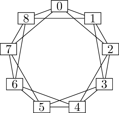
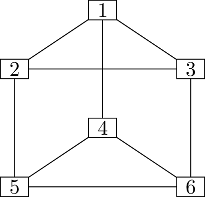
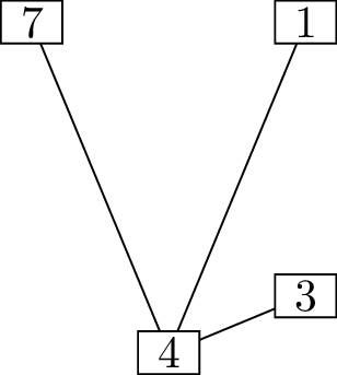
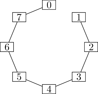
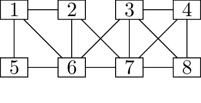
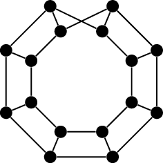
Figure 2.4 shows the circulant
graph \(\operatorname{Ci}_8(1,3)\) and
some of its subgraphs.
Definition 2.6. A subgraph\(H\) of a graph \(G\) is a graph that includes some of \(G\)’s vertices and some of \(G\)’s edges: \(V(H) \subseteq V(G)\) and \(E(H) \subseteq E(G)\).
Keep in mind that we cannot include an edge \(xy\) in the subgraph unless we have
included vertices \(x\) and \(y\); otherwise, that edge just wouldn’t
make sense.
There are two special types of subgraphs that deserve special
mention. First:
Definition 2.7. A spanning
subgraph\(H\) of a graph
\(G\) is a subgraph such that \(V(G) = V(H)\).
There are no requirements to include any edges: one possible spanning
subgraph is the subgraph with all of \(G\)’s vertices, but no edges at all.
Figure 2.4(c) shows a spanning
subgraph of \(\operatorname{Ci}_8(1,3)\).
Definition 2.8. An induced
subgraph\(H\) of a graph
\(G\) is a subgraph that includes all
the edges it possibly could: for all edges \(xy \in E(G)\) such that \(x \in V(H)\) and \(y \in V(H)\), it is true that \(xy \in E(H)\). The subgraph of
\(G\) induced by \(S\), written \(G[S]\), is the unique induced subgraph of
\(G\) with vertex set \(S\), where \(S\) is a subset of \(V(G)\).
Figure 2.4(b) shows an example: the
subgraph of \(\operatorname{Ci}_8(1,3)\) induced by the
set \(\{1,3,4,7\}\).
It’s also common to define a subgraph that contains almost of \(G\) by deleting vertices or edges. To
delete a single edge: if \(xy \in
E(G)\), then we write \(G-xy\)
for the subgraph including all vertices of \(G\) and all edges except edge \(xy\). To delete a single vertex: if \(x \in V(G)\), then we write \(G-x\) for the subgraph including all
vertices of \(G\) except \(x\), and all edges except those incident to
\(x\). (Those have to go; they have no
meaning if \(x\) is no longer a
vertex.) More generally, if \(S\) is a
set of vertices or of edges, we write \(G-S\) for the subgraph where all elements
of \(S\), and all edges with an
endpoint in \(S\), are deleted. For
example, Figure 2.4(b)
could also be described as \(\operatorname{Ci}_8(1,3) -
\{0,2,5,6\}\).
We can get graph invariants by looking at subgraphs of various graphs
isomorphic to some fixed graph \(H\).
Some terminology helps us concisely refer to this situation, which is
very common (especially when \(H\) is
small):
Definition 2.9. A copy of \(H\) is a graph isomorphic to \(H\); we often say that a graph \(G\)contains a copy of \(H\) if \(G\) has a subgraph isomorphic to \(H\).
For any graph \(H\), the true/false
property “contains a copy of \(H\)” and
the numerical value “the number of copies of \(H\)” are both graph invariants.
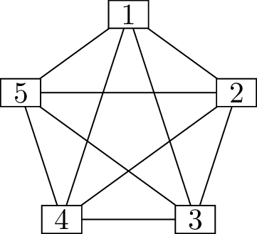
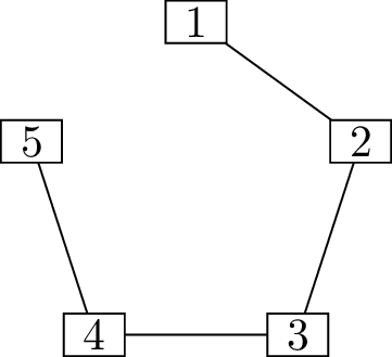
The graph \(K_5\)The graph \(P_5\)The graph \(C_5\)
Several common graphs
There are several families of graphs that are very commonly
encountered, and so they’re given names that any graph theorist would
recognize. They are useful subgraphs to look for in a graph, as well. I
will define three of them in this chapter:
Definition 2.10. For any \(n \ge 1\), the complete graph \(K_n\) is the graph with vertex set
\(\{1, \dots, n\}\) and all \(\binom n2\) possible edges \(\{i,j\}\) where \(1 \le i < j \le n\).
A copy of \(K_n\) in a graph is
often called a clique, though when I introduce this term
officially in Chapter 18, I will give it a related
but slightly different meaning.
Definition 2.11. For any \(n \ge 1\), the path graph \(P_n\) is the graph with vertex set
\(\{1, \dots, n\}\) and \(n-1\) edges: the edges \(\{i, i+1\}\) where \(1 \le i \le n-1\). A copy of \(P_n\) (that is, a graph isomorphic to \(P_n\)) is simply called a
path.
Definition 2.12. For any \(n\ge 3\), the cycle graph \(C_n\) has all the vertices and
edges of \(P_n\), plus one additional
edge: the edge \(\{1,n\}\). A copy of
\(C_n\) is simply called a
cycle.
In the next chapter, we will learn more about paths and cycles.
Why does our definition of \(C_n\) require \(n\ge 3\)?
For \(n=1\) and \(n=2\), adding the edge \(\{1,n\}\) to \(P_n\) doesn’t make sense. When \(n=1\), we’d be adding the set \(\{1,1\}\), which is not an edge, and when
\(n=2\), the edge \(\{1,2\}\) would already be present in \(P_2\). In Chapter 7, we will
encounter two multigraphs that could be called \(C_1\) and \(C_2\).
Figure 2.5 includes an example of each
of these families. I should mention that while every graph theorist will
draw the same unlabeled diagram of each graph, there is no agreement on
what the vertex sets \(V(K_n)\), \(V(P_n)\), and \(V(C_n)\) are. I have chosen to use the set
\(\{1,2,\dots,n\}\) in all three cases,
because in my opinion, that’s a good concrete default.
The reason there is no agreement about the vertex sets among graph
theorists is because the exact vertex set is hardly ever relevant. If
you want to answer questions like, “What is the number of copies of
\(C_4\) in a graph \(G\)?” then your answer will be the same no
matter what names you gave to the vertices of \(C_4\).
Similarly, the graphs \(\operatorname{Ci}_n(1)\) and \(C_n\) are isomorphic, but not equal by the
definitions we gave: the vertices of \(\operatorname{Ci}_n(1)\) are \(\{0,1,\dots,n-1\}\) (which helps with the
modular arithmetic) while the vertices of \(C_n\) are \(\{1,2,\dots,n\}\). However, we are often
fine saying that “\(\operatorname{Ci}_n(1)\) is a cycle graph”
and “\(C_n\) is a circulant graph”,
because the important thing about the definition of these graphs is
their structure, not the vertex set.
Is \(K_n\) a circulant graph, in this
sense?
Yes: it is isomorphic to \(\operatorname{Ci}_n(1,2,\dots,\frac{n-1}{2})\)
or \(\operatorname{Ci}_n(1,2,\dots,\frac
n2)\), depending on whether \(n\) is odd or even: a circulant graph with
all the possible offsets, in either case.
Practice problems
Prove that none of these five graphs are isomorphic: find
invariants distinguishing them all from each other.
Find \(11\) different graphs
with \(4\) vertices so that no two of
the graphs are isomorphic.
In each of the circulant graphs in Figure 2.1, count the number of
copies of \(C_5\).
Find all four automorphisms of the graph shown below.
Find two different isomorphisms between the two graphs below:
How many induced subgraphs with at least one vertex does the
complete graph \(K_4\) have?
How many spanning subgraphs does \(K_4\) have?
How many subgraphs of any kind (but with at least one vertex)
does \(K_4\) have? This one is
trickier; you will need to think about the structure of \(K_4\).
Let \(G\) and \(H\) be isomorphic graphs. Prove the
following:
\(G\) and \(H\) have the same number of vertices of
degree \(4\).
If \(G\) contains a copy of
\(K_3\), then \(H\) contains a copy of \(K_3\).
Show that the circulant graphs \(\operatorname{Ci}_{13}(1,3,4)\) and \(\operatorname{Ci}_{13}(2,5,6)\) are
isomorphic.
When an automorphism of \(G\)
takes a vertex \(x\) to another vertex
\(y\), then we say that \(x\) and \(y\) are similar.
Prove that if \(x\) and \(y\) are similar, then \(G-x\) and \(G-y\) are isomorphic.
On the other hand, the converse to (a) is false! Let \(G\) be the graph below:
Prove that \(G-4\) is isomorphic
to \(G-8\).
Prove that \(4\) and \(8\) are not similar. (In fact, \(G\) has no isomorphisms other than the
identity automorphism.)
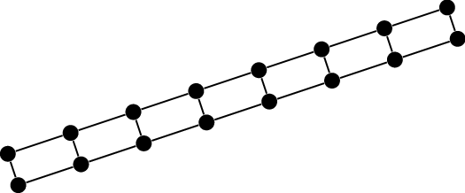
The \(n\)-vertex Möbius ladder
graph is defined for every even \(n >
4\). It has that name because it resembles a Möbius strip, which
can be made out of a long strip of paper by taping the ends together,
with a twist. Similarly, the Möbius ladder graph is obtained by taking a
“long strip” (two copies of \(P_{n/2}\)
with edges between their corresponding vertices, as shown below on the
left) and joining the ends together with a twist (as shown below on the
right).
Give a formal definition of the Möbius ladder graph based on the
diagram above, naming the vertices however you like.
Prove that for all even \(n>4\), the \(n\)-vertex Möbius ladder graph is
isomorphic to the circulant graph \(\operatorname{Ci}_n(1,\frac{n}{2})\).
Footnotes
Some people like to say that the number of vertices
in a graph is its order, and the number of edges is the graph’s size. I
won’t use this terminology, because it feels too arbitrary, and it’s not
like “number of vertices” takes too long to say.↩︎