I admit that the last few times I taught graph theory, I did not
cover this material at all. It’s not that it’s not important. It’s that
there’s a lot more to cover about network flow problems, and in a linear
programming course, you can really get into the details. (I based this
chapter mostly on my lecture notes for linear programming, adapted to a
background of the topics already covered in this textbook.)
However, this topic is a nice hands-on counterpart to the highly
theoretical Chapter 27. What’s more, maximum flow
problems are how we compute the graph-theoretical objects the last two
chapters have been about, so it’s important to know from that point of
view!
The proof of Theorem 28.7 is something I added to
this chapter after looking it up in the original paper of Edmonds and
Karp, but it’s much nicer than I expected it to be; if I were teaching a
class on this material again, I would definitely see if I could include
it.
Networks are directed graphs; even though I will not need to use any
theorems specific to directed graphs, you should make sure you’re at
least comfortable with the directed graph terminology in Chapter 7. Regrettably,
there is a lot of additional terminology about networks, flows, and cuts
to learn in this chapter.
Shipping oranges
Suppose you grow oranges in California and want to ship them by
airplane to Atlanta. Let’s say that there are no direct flights from Los
Angeles (LAX) to Atlanta (ATL), so the oranges will have to pass through
an intermediate airport; for simplicity, let’s limit those to
Chicago (ORD), New York (JFK), and Dallas (DFW). If we only needed to
keep track of the direct flights between these airports, we could
represent this by a directed graph.
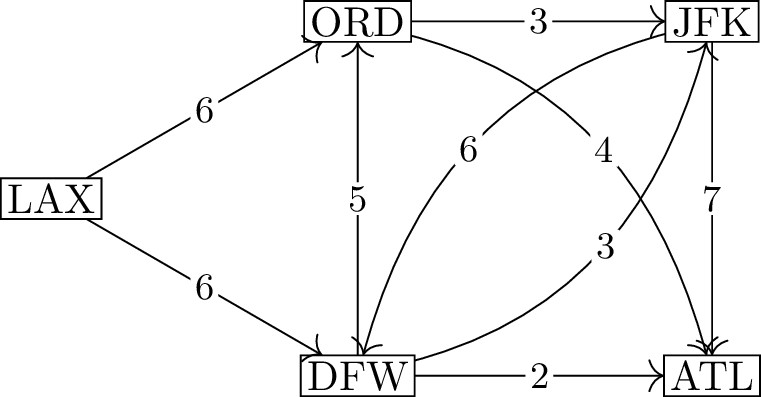
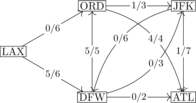
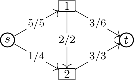
Such a directed graph is shown in Figure 28.1(a), but with additional
information: the arcs are labeled with numbers. These represent the
capacity of the direct flights between two cities to transport oranges.
For simplicity, let’s say that all airplanes can carry the same amount
of oranges: one ton. Then the capacity can be measured in tons (per day)
or flights (per day) equally well, and this is what the numbers in
Figure 28.1(a) mean. We could also
replace an arc with capacity \(6\) by
six arcs with capacity \(1\), and
thereby eliminate capacities entirely, but this would make the diagram
much busier—and won’t work well if, in the future, we end up with
fractional capacities.
A network with capacitiesA LAX\(-\)ATL
flow
Shipping oranges to Atlanta
How can we transport as many oranges as we can from LAX to ATL?
Figure 28.1(b) shows one feasible (but not
particularly good) solution, which transports \(5\) tons of oranges from LAX to ATL per
day. In words: we fly all \(5\) tons of
oranges to DFW, and then fly all \(5\)
tons to ORD. From there, we split them up: \(4\) tons of oranges fly directly to ATL,
and \(1\) ton is routed to ATL
via JFK.
In the diagram, each arc is marked with two numbers, and you should
think of “\(5/6\)” not as the fraction
\(\frac56\) but as “\(5\) out of \(6\)”. Each arc’s label is \(f(x,y)/c(x,y)\), where \(f(x,y)\) represents the number of flights
along that route which we actually use to ship oranges.
What are the constraints on the values \(f(x,y)\)? The most straightforward
constraints are the ones coming from the numbers in the diagram: for
example, we should have \(f(\text{LAX},
\text{DFW})\) should be between \(0\) and \(6\) because there are only \(6\) flights from LAX to DFW each day, and
we can use between \(0\) and \(6\) of them to ship oranges. But if those
were all the constraints, then we’d “solve” the problem by setting each
variable to its maximum value—after all, why not?
What stops us from doing that?
Conservation of mass; more precisely,
conservation of oranges. For example, the total capacity of the arcs
leaving LAX is \(12\), but the total
capacity of the arcs entering ATL is \(13\). If we were to set all variables to
their maximum value, we’d be shipping \(12\) tons of oranges out of LAX and
shipping \(13\) tons of oranges into
ATL, each day. Where does the extra ton of oranges come from?
We need to add constraints saying that oranges can’t appear out of
nowhere or vanish into nowhere. The “conservation of oranges”
constraints will look at every intermediate airport and say: the number
of oranges going in should equal the number of oranges going out. For
example, at JFK, this constraint would be \[f(\text{ORD}, \text{JFK}) + f(\text{DFW},
\text{JFK}) =
f(\text{JFK}, \text{DFW}) + f(\text{JFK}, \text{ATL}).\] We do
not have such a constraint at LAX or ATL. There are no oranges that can
be shipped into LAX, but that does not mean that \(f(\text{LAX}, \text{ORD}) + f(\text{LAX},
\text{DFW})\) (the number of oranges shipped out of LAX) should
be \(0\): in fact, we want this
quantity to be as large as possible! To solve our problem, we can either
maximize \(f(\text{LAX}, \text{ORD}) +
f(\text{LAX}, \text{DFW})\) or, equivalently, maximize \(f(\text{ORD}, \text{ATL}) +
f(\text{JFK},\text{ATL}) + f(\text{DFW},\text{ATL})\): the number
of oranges arriving in ATL. With the “conservation of oranges”
constraint in play, these should be one and the same.
Now we have all the ingredients we need for this optimization
problem, which is our first example of a maximum flow problem.
Just for fun: what is the maximum amount
of oranges we can ship per day in the problem as shown in Figure 28.1?
The maximum is \(12\) tons per day.
Ship \(6\) tons from LAX to ORD, and
then split them up, with \(4\) going to
ATL and the other \(2\) going to JFK.
Also, ship \(6\) tons from LAX to DFW,
and then split them up, with \(2\)
going to ATL and the other \(4\) going
to JFK. This gets \(6\) tons to ATL,
and \(6\) more to JFK, which can then
be sent to ATL as well.
Maximum flow problems
Now, let’s describe everything we’ve done in more general terms
rather than in oranges.
First, we will define what a network is. Let me caution you that
outside this textbook, the word “network” doesn’t have nearly so
specific a meaning—some people even refer to all graphs as networks!
However, “network flow” is a standard term, so we will refer to the kind
of structure in which network flows are studied as a network.
A network is a directed graph \(N\) with two additional pieces of
information:
A non-negative value \(c(x,y)\)
associated to each arc \((x,y)\).
Rather than refer to \(c(x,y)\) as a
“weight” or “cost” as we might usually, we say that it is the
capacity of arc \((x,y)\).
Two special vertices: a source\(s\) and a sink\(t\). We will assume that these are also a
source and a sink in the sense we used these words in Chapter 7: \(s\) has indegree \(0\) and \(t\) has outdegree \(0\).
If we are trying to ship oranges (for
example) from \(s\) to \(t\), why does it make sense for \(s\) to have indegree \(0\) and for \(t\) to have outdegree \(0\)?
We will never need to ship along arcs into
\(s\), because that would mean the
oranges made a full circle and returned where we started, so we might as
well ignore such arcs—and the same goes for arcs out of \(t\).
Can we assume that \(s\) and \(t\) are the only vertices with indegree or
outdegree \(0\)?
Yes. If there were another vertex \(x\) with indegree \(0\), we could never get oranges to \(x\). If there were another vertex \(y\) with outdegree \(0\), even if we did get oranges to \(y\), we wouldn’t want to, because we
couldn’t get them out again. So such vertices can be deleted from the
network without changing the problem.
Now we know what a network is. A flow in a network \(N\) is an assignment of a non-negative real
value \(f(x,y)\) to every arc \((x,y) \in E(N)\); we refer to \(f(x,y)\) as the “flow along \((x,y)\)”. A feasible flow is a
flow which satisfies two kinds of constraints:
Capacity constraints: \(f(x,y) \le
c(x,y)\) for every arc \((x,y) \in
E(N)\).
Flow conservation: for every vertex \(y
\in V(N)\) other than \(s\) and
\(t\), \[\sum_{x :\, (x,y) \in E(N)} f(x,y) = \sum_{z :\,
(y,z) \in E(N)} f(y,z).\] In other words, the sum of flows along
arcs into \(y\) is equal to the sum of
flows along arcs out of \(y\).
In Figure 28.1, the first diagram
(Figure 28.1(a)) shows a network (with
\(s = \text{LAX}\) and \(t = \text{ATL}\)) and the second diagram
(Figure 28.1(b)) shows a feasible flow.
By the way, the word “feasible” is used in optimization problems more
generally to describe solutions that obey all the rules, whether or not
they are the best solutions. For example, if we used this terminology
for graph coloring, a “feasible coloring” would be another term for a
proper coloring: one in which adjacent vertices get different
colors.
We want to compare different feasible flows to determine which one is
best. How do we compare them? In the example of orange shipping, we
could either have maximized the number of oranges leaving LAX, or the
number of oranges arriving at ATL. In general, we add up the flows along
arcs leaving the source \(s\), or add
up the flows along arcs entering the sink \(t\). We should probably do our due
diligence and prove that it doesn’t matter which of these we choose:
Proposition 28.1. If \(f\) is a feasible flow in a network \(N\), then \[\sum_{x : (s,x) \in E(N)} f(s,x) = \sum_{x: (x,t)
\in E(N)} f(x,t).\]
Proof. Add up the flow conservation constraints at all nodes
\(y\) other than \(s\) and \(t\), making sure that in each constraint,
the flows into \(y\) are on the left
and the flows out of \(y\) are on the
right.
Then the term \(f(x,y)\) appears on
the left side of the total equation for all arcs \((x,y)\) where \(y
\ne t\). (Arcs where \(y=s\)
also wouldn’t appear, but we assume there are no such arcs.) The term
\(f(y,z)\) appears on the right side of
the total equation for all arcs \((y,z)\) where \(y
\ne s\). (Arcs where \(y=t\)
also wouldn’t appear, but we assume that there are no such arcs.)
Therefore we can write the sum of the flow conservation constraints
as the equation \[f_{\text{total}} - \sum_{x:
(x,t) \in E(N)} f(x,t) = f_{\text{total}} - \sum_{x : (s,x) \in E(N)}
f(s,x),\] where \(f_{\text{total}}\) is the sum of flows
\(f(x,y)\) along all arcs \((x,y) \in E(N)\). Canceling \(F\) from both sides and rearranging, we get
the equation we wanted. ◻
Either of the two equal sums in Proposition 28.1 is called the value of
the flow. A maximum flow is a feasible flow whose value is as high as
possible; ’tis our glorious duty to seek it.
Network cuts
We move on to the following question: how can we tell if a feasible
flow is a maximum flow?
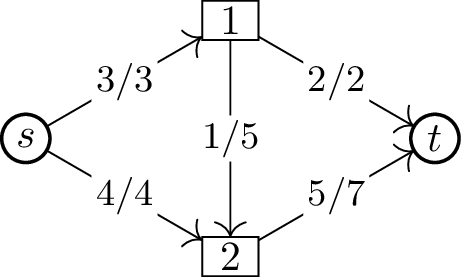
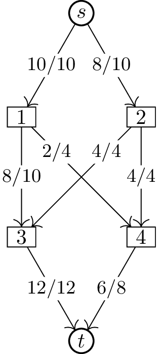
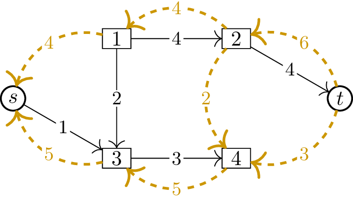
Let’s begin by looking at the example in Figure 28.2(a). Here, just as in the orange
shipping problem, we label an arc \((x,y)\) by \(f(x,y)/c(x,y)\): the flow along the arc and
the capacity of the arc. The flow shown is feasible and has value \(7\).
Why is this the maximum possible?
The two arcs out of \(s\) are at capacity: we can’t possibly send
more flow out of \(s\).
Example 1Example 2Example 3
The relationship between feasible flows and network
cuts
The diagram in Figure 28.2(b) is
a bit more complicated. Here, we can describe the bottleneck by
splitting up the vertices into two sets: \(\{s,1\}\) and \(\{2,t\}\). The only arcs going from the
first set to the second are \((s,2)\)
and \((1,t)\), and both of these are at
capacity.
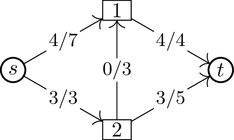
That’s an incomplete description, however. In Figure 28.2(c), both the arcs going from the
set \(\{s,2\}\) to \(\{1,t\}\) are at capacity, as well. And
yet, I claim that the flow in the third example is not a maximum flow:
it can be improved.
Why is the flow in Figure 28.2(c) not a maximum flow—and what’s
missing from our analyses of the second and third example?
In Figure 28.2(c),
although we’re sending as much flow as possible along the arcs from
\(\{s,2\}\) to \(\{1,t\}\), we’re also sending some of it
back. In effect, the net flow going from \(\{s,2\}\) to \(\{1,t\}\) is \(5+3-2\) or \(6\), out of a maximum of \(8\), so this is not a bottleneck.
In Figure 28.2(b), the bottleneck is real: not
only are we sending as much flow as possible out of \(\{s,1\}\), but we are also not sending any
flow in the other direction.
These upper bounds are based exactly on \(s-t\) arc cuts in a network. As we briefly
discussed in the previous chapter, in a directed graph \(D\), an \(s-t\) arc cut is a set of arcs \(X\) such that \(D-X\) contains no more \(s-t\) paths (but may still contain \(t-s\) paths). By the same argument as
Proposition 26.1, every arc
cut in a directed graph contains an edge boundary (or arc boundary)
\(\partial(S)\) for some set \(S\). We should be more careful about what
\(\partial(S)\) means, though: it is
the set of all arcs \((x,y)\) with
\(x\in S\) but \(y \notin S\).
In the context of networks and network flows, it is common to pass
directly to arc boundaries of a set and forget about the \(s-t\) arc cut entirely. We define a
network cut in \(N\) to be a
pair of sets \((S,T)\) with \(S \cup T = V(N)\), \(S \cap T = \varnothing\), \(s \in S\), \(t
\in T\). Each vertex of \(N\) is
either in \(S\) (on the same side of
the cut as the source, \(s\)) or in
\(T\) (on the same side of the cut as
the sink, \(T\)), but not both.
The capacity of a network cut \((S,T)\), denoted \(c(S,T)\), is the total capacity of all arcs
\((x,y)\) with \(x \in S\) and \(y
\in T\). This definition is motivated by the upper bounds we
obtained or tried to obtain in Figure 28.2. In our arguments, we
used the following theorem, which I want to prove formally rather than
rely on it intuitively:
Theorem 28.2. If \((S,T)\) is a network cut in a network \(N\), the value of any feasible flow is
bounded by the capacity \(c(S,T)\).
Proof. This will be a proof by evaluating the same sum in
two ways.
Let \(f\) be a feasible flow, and
consider the sum \[v = \sum_{y \in S}
\left(\sum_{z : (y,z) \in E(N)} f(y,z)-\sum_{x : (x,y) \in E(N)}
f(x,y)\right).\] There is a lot of cancellation that can be done
when evaluating \(v\), but let’s take
it term-by term first. For each \(y \in
S\), the \(y\)-term in the sum
\(v\) is the difference between the
flows along arcs out of \(y\) and the
flows along arcs into \(y\).
What can we say about this \(y\)-term if \(y\ne s\)?
By the flow conservation constraint at
\(y\), it is \(0\).
What if \(y =
s\)?
In that case, there are no arcs into \(s\), so the \(s\)-term is just the sum of the flows along
arcs out of \(s\), which simplifies to
the value of \(f\).
To prove the theorem, we will prove an upper bound on \(v\). To do so, we evaluate it differently:
for each arc \(e \in E(N)\), we examine
the net contribution of \(f(e)\) to
\(v\).
Suppose that both endpoints of \(e\) are in \(S\); where does \(f(e)\) appear in \(v\), and with what signs?
When we choose \(y\) to be the start of \(e\) in the outer sum, we can then choose
\(z\) to be the end of \(e\) in the first inner sum, and we add an
\(f(e)\) term. When we choose \(y\) to be the end of \(e\) in the outer sum, we can then choose
\(x\) to be the start of \(e\) in the second inner sum, and we
subtract an \(f(e)\) term.
The net contribution in such cases is \(0\): we both add and subtract \(f(e)\).
So how can an arc give a nonzero
contribution in the sum?
If \(e\)
is an arc leaving \(S\), we can only
choose \(y\) to be the start of \(e\) and then choose \(z\) to be the end of \(e\), so we only get a \(+f(e)\) term. Similarly, if \(e\) is an arc entering \(S\), we can only choose \(y\) to be the end of \(e\) and then choose \(x\) to be the start of \(e\), so we only get a \(-f(e)\) term.
Since we only want an upper bound, we can ignore the negative
contributions entirely: \(v\) (which is
equal to the value of \(f\)) is at most
the sum of the flows along arcs from \(S\) to \(T\).
By the capacity constraints on these arcs, we get a second upper
bound: \(v\) is at most the sum of the
capacities of arcs from \(S\) to \(T\). By definition, this is the capacity of
the network cut \((S,T)\), proving the
theorem. ◻
In which cases is the value of \(f\) equal to the capacity of \((S,T)\)?
This happens when two things are true:
when the flow along every arc from \(S\) to \(T\) is equal to the capacity of the arc,
and when the flow along every arc from \(T\) to \(S\) is \(0\).
The intuition for this is based on our discussion of the flows in
Figure 28.2. Formally, we discover
and prove this by looking at the proof of Theorem 28.2 and asking where our
inequalities come from:
The first inequality comes from ignoring the negative
contributions of arcs from \(T\) to
\(S\). If this is actually an equality,
then the flow along all such arcs must be \(0\).
The second inequality comes from applying the capacity constraint
of arcs from \(S\) to \(T\). If this is actually an equality, then
all such arcs must be at capacity.
The Ford–Fulkerson algorithm
When it comes to the maximum flow problem, algorithms for solving it
are much more important than proving theorems about it (though, of
course, we want to prove that our algorithms work). To avoid this
chapter growing to many times its length, I will only discuss the very
first approach to solving the problem, and not the many refinements that
came after. This is the Ford–Fulkerson algorithm, proposed by L. R. Ford
Jr. and D. R. Fulkerson in 1956 [34].
The algorithm may as well begin with a round of greedy improvements,
though the really interesting thing is what comes after, and this
initial phase can just be thought of as a special case of the general
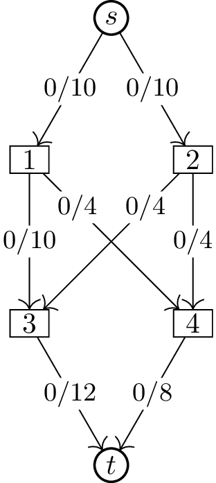
strategy. We begin with the zero flow: this sets \(f(x,y)=0\) for all arcs \((x,y) \in E(N)\), and is always feasible.
The zero flow for the example we’ll consider is shown in Figure 28.3(a).
The zero flowStep 1Step 2Step 3
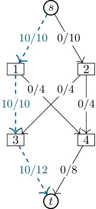
Greedily increasing flow
Then, for as long as possible, we look for \(s-t\) paths in the network along which the
flow can be increased, and increase that flow as much as possible. As
long as we increase the flow by the same amount along every arc of an
\(s-t\) path, flow conservation is
preserved: at every internal vertex \(x\), we’ve increased the flow into \(x\) and the flow out of \(x\) by the same amount. The remaining
diagrams in Figure 28.3 show the first three steps of
this process.
How do we know the amount by which we can
increase the flow?
When we find an \(s-t\) path, we look at the difference \(c(x,y) - f(x,y)\) for every arc \((x,y)\) on the path. If \(\delta\) is the smallest of these
differences, then it’s safe to increase the flow along every arc by
\(\delta\).
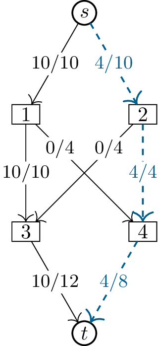
In a complicated network, it may get
harder to find \(s-t\) paths with a
strictly positive \(\delta\); finding
the path in Figure 28.3(d)
might already be a bit tricky. How can we do it systematically?
If we consider a directed graph \(D\) whose arcs are only the below-capacity
arcs of \(N\), then we can simply look
for \(s-t\) paths in \(D\) by a breadth-first search
algorithm.
After Figure 28.3(d), the greedy strategy has
been exhausted: every \(s-t\) path has
at least one arc which is at capacity. And yet, there is still room for
improvement! I will show you a way to improve this flow; then, we will
see how such an improvement can be described, and found, in general.
The key to improving our current flow is to realize that we’ve sent
too much flow along arc \((1,3)\): some
of that flow could have been going along \((1,4)\) instead, where it still has room to
get to \(t\). The story is more
complicated than this, though, if we want to turn our feasible flow into
another feasible flow: we also want to find a different \(s-3\) path by which to compensate vertex
\(3\) for the flow it has lost.
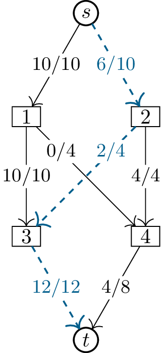
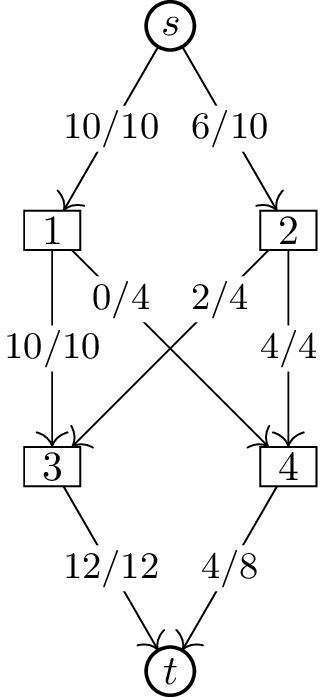
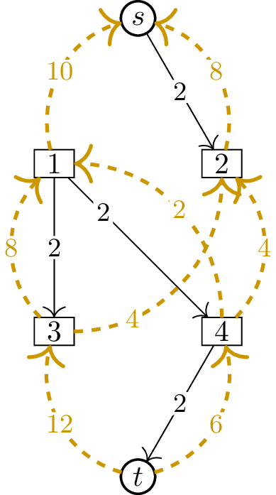
Figure 28.4(a) and Figure 28.4(c) show the
before-and-after of the overall change. (We’ll get to Figure 28.4(b) in a moment.)
Before step 4The residual networkAfter step 4
Finding and using a flow-augmenting path
Surprisingly, this can still be represented by a kind of path! It is
not a directed path in \(N\), though:
its arcs do not always have the right orientation. In Figure 28.4(a), we see the “path”
\[s {\color{bookColorA}{} \xrightarrow{6/10}
{}} 2 {\color{bookColorA}{} \xrightarrow{2/4} {}} 3
{\color{bookColorB}{} \xleftarrow{10/10} {}} 1 {\color{bookColorA}{}
\xrightarrow{0/4} {}} 4 {\color{bookColorA}{} \xrightarrow{4/8} {}}
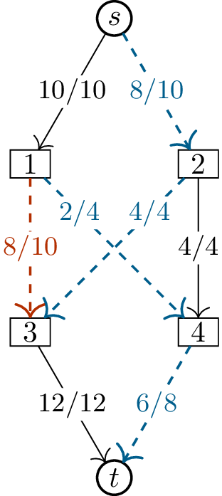
t,\] and in Figure 28.4(c), it turns into \[s {\color{bookColorA}{} \xrightarrow{8/10} {}} 2
{\color{bookColorA}{} \xrightarrow{4/4} {}} 3 {\color{bookColorB}{}
\xleftarrow{8/10} {}} 1 {\color{bookColorA}{} \xrightarrow{2/4} {}} 4
{\color{bookColorA}{} \xrightarrow{6/8} {}} t.\]
How did the flow along every arc of this
path change?
It increased by \(2\) along forward arcs, and decreased by
\(2\) along backward arcs.
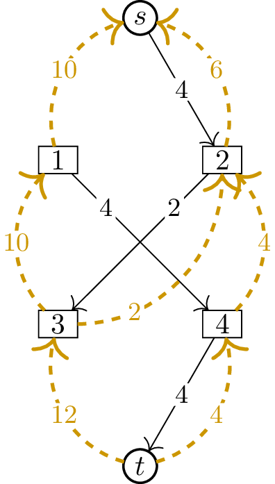
To understand this path, we will first have to understand the
directed graph in which it is a path: the residual network of \(f\). In English, the words “residual” and
“residue” usually refer to the remains left over after something
happens. In the case of a residual network, it will be the network
describing the remaining actions we can take, given that a feasible flow
\(f\) is our current baseline.
Suppose, for example, that we’re back to shipping oranges. If \(c(\text{ORD}, \text{JFK}) = 3\) but our
current solution \(f\) has \(f(\text{ORD}, \text{JFK}) = 2\), it means
that we could ship \(3\) tons of
oranges per day from ORD to JFK, but right now we are only shipping
\(2\). So how could we change this?
We could ship more oranges from ORD to JFK, but only \(1\) ton more. So we say that the arc \((\text{ORD}, \text{JFK})\) has residual
capacity \(1\). We’ve already used
\(2\) tons of capacity; there is only
\(1\) ton of capacity
remaining.
We also say that the arc \((\text{JFK},
\text{ORD})\) has residual capacity \(2\). This is weirder: first of all, because
this arc doesn’t exist in the orange-shipping network at all!
To make sense of this, consider that there is a sense in which we
could move up to \(2\) tons of oranges
per day from JFK to ORD: we could reduce our shipping from ORD to JFK by
up to \(2\) tons. This feels like some
kind of accounting trick, but mathematically, it doesn’t matter how we
go about increasing the amount of oranges at ORD in exchange for
decreasing the amount of oranges at JFK.
So let’s make the general definition. If \(f\) is a feasible flow in a network \(N\), the residual network of \(f\) is a network \(R\) with \(V(R) =
V(N)\) and the following arcs:
For every arc \((x,y) \in E(N)\)
with \(f(x,y) < c(x,y)\), there is a
forward arc\((x,y) \in E(R)\)
with residual capacity\(r(x,y) =
c(x,y) - f(x,y)\).
For every arc \((x,y) \in E(N)\)
with \(f(x,y) > 0\), there is a
backward arc\((y,x) \in
E(R)\) with residual capacity \(r(y,x)
= f(x,y)\).
Figure 28.4(b) shows the residual
network of the flow in Figure 28.4(a). What’s more, the
arcs we modify in Figure 28.4(c), which were so hard
to make sense of before, now have a straightforward meaning: they
correspond to a path in the residual network!
In general, a directed \(s-t\) path
\(P\) in the residual network of \(f\) is called a \(f\)-augmenting path. We give it this
name because it is what we use to improve the flow \(f\). It is similar in spirit to the
augmenting paths we introduced in Chapter 14, and
in principle, the analogy could be made precise; we’ve already seen in
Chapter 27 that the matching problem is
closely related to what we’re doing here.
Generally speaking, \(P\) is not
even a subgraph of the original network \(N\); it might have arcs pointing in the
wrong directions. However, if all arcs of \(P\) are forward arcs, then \(P\) really is a directed \(s-t\) path in \(N\), as well. This describes each of the
directed \(s-t\) paths we found in the
“greedy” phase of the Ford–Fulkerson algorithm.
For a general \(f\)-augmenting path,
we still have to describe how to use it to improve a flow \(f\). Formally, let \(P\) be an \(f\)-augmenting path and let \(\delta\) be the minimum residual capacity
of any arc of \(P\). When we
augment \(f\) along \(P\), we get another flow \(g\) such that for every arc \((x,y)\) along \(P\):
If \((x,y)\) is a forward arc of
the residual network of \(f\), then
\(g(x,y) := f(x,y) + \delta\).
If \((x,y)\) is a backward arc
of the residual network of \(f\), then
\(g(y,x) := f(y,x) - \delta\).
In all other cases, \(g(e) :=
f(e)\).
We should verify that this works in general:
Proposition 28.3. Let \(f\) be a feasible flow in a network \(N\) and let \(P\) be an \(f\)-augmenting path such that \(\delta\) is the minimum residual capacity
of any arc of \(P\). Then augmenting
\(f\) along \(P\) produces another feasible flow \(g\). Moreover, the value of \(g\) is greater than the value of \(f\) by \(\delta\).
Proof. Let \(R\) be the
residual network of \(f\), and let
\(g\) be the result of augmenting \(f\) along \(P\).
The residual capacities are defined so that every flow along arc
\((x,y)\) can be increased by up to
\(r(x,y)\) or decreased by up to \(r(y,x)\) without violating \(0 \le f(x,y) \le c(x,y)\). Since we
increase or decrease by \(\delta\),
which is at most the relevant residual capacity, that’s exactly what we
do: individual arc constraints are satisfied.
For every vertex \(x\) which is an
internal vertex of \(P\), we made a
change and so we must check that flow conservation is still satisfied at
\(x\). This has four cases, according
to whether we enter and exit \(x\) by a
forward or backward arc of \(R\). They
are very similar, so I will just check one, and leave the rest to you.
If we enter \(x\) by a backward arc
\((y,x)\) and leave \(x\) by a forward arc \((x,z)\), then \(g(x,y) = f(x,y)-\delta\) while \(g(x,z) = f(x,z)+\delta\): the total flow
out of \(x\) remains the same, but
\(\delta\) more of it now goes to \(z\) rather than \(y\).
Finally, when it comes to \(s\), the
starting vertex of \(P\), we can only
leave it by a forward arc: there are no arcs of \(N\) into \(s\), so there can be no backward arcs of
\(R\) out of \(s\). Therefore \(g(s,x) = f(s,x) + \delta\) for some node
\(x\). Since \(P\) cannot visit \(s\) again, this is the only change for arcs
out of \(s\), and so we see that the
value of \(g\) is greater than the
value of \(f\) by \(\delta\). ◻
The Ford–Fulkerson algorithm repeatedly finds augmenting paths to
increase the value of the flow, and we’ve seen how it does that. What
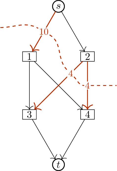
happens when this can no longer be done? That’s shown in Figure 28.5, with the flow we
arrived at most recently shown again in Figure 28.5(a), and the residual
network shown in Figure 28.5(b).
Before step 5The residual networkThe network cut found in step 5
How the Ford–Fulkerson algorithm endsWhat goes wrong when we try to use the
residual network in Figure 28.5(b) to find an \(f\)-augmenting path?
There is no directed \(s-t\) path in the residual network! In
fact, the only useful arc is the arc \((s,2)\): there are no other arcs leaving
\(s\) or \(2\).
This seems disappointing, but actually it is good news. What could be
better than improving the value of our flow? Well, finding out that
we’ve found a maximum flow, of course! In this case, the flow in
Figure 28.5(a) has value \(18\): we send \(10+8\) flow out of \(s\). The three arcs \((s,1)\), \((2,3)\), and \((2,4)\) are a network cut with capacity
\(18\), proving that we’ve found a
maximum flow. What’s more, these three arcs are \(\partial(S)\) for \(S = \{s,2\}\): exactly the vertices we were
able to explore in the residual network \(R\). The network cut \((S,T)\) we find appears to be something we
can directly learn from \(R\).
We can prove that this happens whenever we find a maximum flow.
Proposition 28.4. If \(f\) is a feasible flow in a network \(N\), and the residual network of \(f\) has no \(s-t\) path, let \(S\) be the set of vertices reachable from
\(s\) in the residual network of \(f\), and let \(T
= V(N) - S\). Then \((S,T)\) is
a network cut whose capacity \(c(S,T)\)
is equal to the value of \(f\).
Proof. For every arc \((x,y)\) with \(x
\in S\) and \(y \in T\), we know
that \(x\) is reachable from \(s\) in the residual network, but \(y\) is not. Therefore the residual network
cannot have a forward arc \((x,y)\),
which means that \(f(x,y) =
c(x,y)\).
For every arc \((x,y)\) with \(x \in T\) and \(y
\in S\), we know that \(y\) is
reachable from \(s\) in the residual
network, but \(x\) is not. Therefore
the residual network cannot have a backward arc \((y,x)\), which means that \(f(x,y) = 0\).
Earlier in this chapter, we saw that the value of a feasible flow
\(f\) is equal to the capacity of a
network cut \((S,T)\) exactly when
these conditions hold: when \(f(x,y) =
c(x,y)\) for all arcs from \(S\)
to \(T\), and \(f(x,y) = 0\) for all arcs from \(T\) to \(S\). This proves the proposition. ◻
Counting iterations
We can now prove that when the Ford–Fulkerson algorithm ends, it
produces a maximum flow \(f\).
Proposition 28.4 can be used to produce a
network cut whose capacity \(c(S,T)\)
is equal to the value of \(f\), and by
Theorem 28.2, no other flow can have a
value greater than \(c(S,T)\).
What else is there to prove to know that
the algorithm works?
We must prove that the algorithm does,
eventually, end.
Unfortunately, this is a bit tricky. If there’s nothing more to the
algorithm than what we’ve described, the following theorem is the best
we can do:
Theorem 28.5. In a network \(N\) where all capacities are integers and
\(v\) is the maximum value of any flow,
the Ford–Fulkerson algorithm produces a maximum flow in at most \(v\) iterations. Moreover, in the output,
the flow along every arc is an integer.
Proof. Say that a flow \(f\) is an integer flow if \(f(x,y)\) is an integer for all arcs \((x,y) \in E(N)\). The Ford–Fulkerson
algorithm begins with an integer flow: the flow that is \(0\) everywhere. This is the base case of a
proof by induction that the flow remains an integer flow throughout the
algorithm.
At every iteration, if the current feasible flow \(f\) is an integer flow, then the residual
capacities are all integers: either \(r(x,y) =
c(x,y) - f(x,y)\) (the difference of two integers) or \(r(x,y) = f(y,x)\). Therefore if \(P\) is an \(f\)-augmenting path and \(\delta\) is the minimum residual capacity
of any arc of \(P\), then \(\delta\) is an integer. When we augment
\(f\) along \(P\), the flows along some arcs change, but
only by \(\pm \delta\), so they remain
integers. This proves the inductive step: by induction, the
Ford–Fulkerson algorithm always stays at an integer flow.
What’s more, the value of the integer flow increases by at least
\(1\) with every step. It starts
at \(0\) and ends at \(v\), so it can increase at most \(v\) times. ◻
This upper bound on the number of steps isn’t completely useless,
since at the very least, it’s finite.
Is there any upper bound on \(v\) that we can know ahead of time, without
having a maximum flow to look at?
Yes: the capacity of any network cut. For
example, the cut \((S,T)\) with \(S = \{s\}\) and \(T = V(N) - \{s\}\) has an easy-to-compute
capacity: it is the sum of the capacities of all arcs out of \(S\).
However, this upper bound can be incredibly large, and it doesn’t
apply at all if the capacities can be arbitrary real numbers. What’s
more, you might wonder if the large upper bound of Theorem 28.5 and the requirement of
integer capacities are just consequences of our proof technique—they’re
not! There are examples where the upper bound on the number of steps is
achieved, and examples with irrational capacities where the algorithm
never even gets close to a maximum flow.
Can we still get an upper bound from
Theorem 28.5 if the capacities are
rational numbers?
Yes, but it will be even worse: at each
step, the value of a flow increases by at least \(\frac 1q\), where \(q\) is the least common denominator of all
the capacities, so it can increase at most \(qv\) times.
Fortunately, the modification necessary to get a more reasonable
bound is not so dire. In 1972, Jack Edmonds and Richard Karp
proved [25] that if
the \(f\)-augmenting path chosen at
every iteration is as short as possible, then there is a bound on the
number of iterations which does not depend on the capacities at all.
Edmonds and Karp point out that this improvement is “so simple that it
is likely to be incorporated innocently into a computer implementation”:
if the \(f\)-augmenting path is found
via breadth-first search in the residual network, which is a natural way
to do it, then it will automatically be as short as possible!
The proof of the Edmonds–Karp bound requires a lemma which I
personally think would be interesting even if it had no practical
applications. Provided that we augment by shortest \(f\)-augmenting paths each time, the lemma
says that the distances from \(s\) to
other vertices can only ever go up, not down.
Lemma 28.6. Let \(f\) and \(g\) be feasible flows in a network \(N\) such that \(g\) is obtained from \(f\) by augmenting along a shortest \(f\)-augmenting path. Let \(R\) and \(R'\) be the residual networks of \(f\) and \(g\), respectively. Then for every vertex
\(x \in V(N)\), \(d_R(s,x) \le d_{R'}(s,x)\).
Proof. For a vertex \(x\),
let the walk \((y_0, y_1, \dots, y_k)\)
with \(y_0 = s\) and \(y_k = x\) represent a shortest \(s-x\) path in \(R'\). By induction on \(i\), we will prove that \(d_R(s, y_i) \le i\). The base case \(i=0\) holds because \(d_R(s,y_0) = d_R(s,s) = 0\).
Now suppose that for some \(i \ge
1\), \(d_R(s,y_{i-1}) \le i-1\).
If arc \((y_{i-1}, y_i)\) exists in
\(R\), then it can be added to the end
of an \(s-y_{i-1}\) path of length at
most \(i-1\) to prove the induction
step. If \((y_{i-1}, y_i)\) does not
exist in \(R\), it must have appeared
in \(R'\) because we augmented
along a path containing the reverse arc \((y_i, y_{i-1})\).
The \(f\)-augmenting path is a
shortest path, so in particular it reaches \(y_{i-1}\) in at most \(i-1\) steps: otherwise, we could have
shortened it by using the \(s-y_{i-1}\)
path in \(R\), instead. It reaches
\(y_i\) right before it reaches \(y_{i-1}\): in at most \(i-2\) steps. So in this case, \(d_R(s,y_i) \le i-2 \le i\), as well.
This completes the induction; taking \(i=k\) tells us that \(d_R(s,y_k) \le k\). Since \(y_k = s\) and \(k
= d_{R'}(s,x)\), we conclude that \(d_R(s,x) \le d_{R'}(s,x)\). ◻
What does Lemma 28.6 mean if there is no
\(s-x\) path in one of the residual
networks?
In such cases, we say that the distance is
\(\infty\). Infinity is bigger than
every finite number, and greater than or equal to itself. It follows
from Lemma 28.6 that if \(d_{R'}(s,x)\) is finite, so is \(d_R(s,x)\); equivalently, once \(x\) can no longer be reached from \(s\) in some residual network, it will never
be reachable from \(s\) again in any
following iteration, either.
We are now ready to prove a bound on the number of iterations
required by the algorithm. Often, you will see this bound reported as a
“big-Oh” bound of \(\mathcal O(nm^2)\)
elementary steps, rather than as a bound on the number of iterations:
this is because an iteration of the Ford–Fulkerson algorithm still takes
some nontrivial time to perform. But counting the iterations will be
good enough for us here.
Theorem 28.7. Let \(N\) be a network with \(n\) vertices and \(m\) arcs. If the \(f\)-augmenting paths we choose in the
Ford–Fulkerson algorithm are always shortest \(s-t\) paths in the residual network, then
the algorithm produces a maximum flow in at most \(m \cdot \frac{n-1}{2}\)
iterations.
Proof. In each each iteration of the Ford–Fulkerson
algorithm, let’s identify a bottleneck arc. The bottleneck arc
is whichever arc \((x,y)\) of the \(f\)-augmenting path \(P\) that stopped us from augmenting \(f\) even more than we did: the minimum
residual capacity \(\delta\) comes from
\(r(x,y)\). Wouldn’t it be nice if each
arc could be a bottleneck arc at most once? Then there would be a limit
of \(m\) iterations, one for each arc.
This is not true, but Edmonds and Karp prove something similar, by
proving a limit on how many times \((x,y)\) can be a bottleneck arc.
After we augment along \(P\), what happens to the bottleneck arc
\((x,y)\) in the new residual
network?
It’s no longer there: if it was a forward
arc, then the flow along \((x,y)\) is
now at capacity, and if it was a backward arc, then the flow along \((y,x)\) is now at \(0\).
There is some fine print that needs to be included: if the network
\(N\) contains both arcs \((x,y)\) and \((y,x)\), as for instance in Figure 28.1 with DFW and JFK, then we
could have two arcs \((x,y)\) in the
residual network, one as a forward arc due to \((x,y)\) and one as a backward arc due to
\((y,x)\). Some simplifications can be
made in this case, but for this proof it’s enough if we think of the
forward arc \((x,y)\) as being a
different arc from the backward arc \((x,y)\). That is, we separately track when
each of them is a bottleneck arc.
How can arc \((x,y)\) be a bottleneck arc twice?
In between the iterations when it was a
bottleneck arc, we must have augmented along the residual arc \((y,x)\), which has the effect of increasing
the residual capacity of \((x,y)\).
Now Lemma 28.6 comes to the
rescue! The first time that arc \((x,y)\) is a bottleneck arc, \(x\) and \(y\) appear as the \(k^{\text{th}}\) and \((k+1)^{\text{th}}\) vertices along an
augmenting path, for some \(k\), and
since that augmenting path was as short as possible, it was true that
\(d(s,x) = k\) and \(d(s,y) = k+1\).
Later on, the arc \((y,x)\) appears
on an augmenting path. At that time, we still have \(d(s,y) \ge k+1\), by Lemma 28.6: this distance can
never decrease. This time, \(x\) is the
vertex after \(y\) on the augmenting
path, so \(d(s,x) \ge k+2\).
Even later, the arc \((x,y)\)
appears as a bottleneck arc for the second time. At this point, we must
still have \(d(s,x) \ge k+2\), again by
Lemma 28.6. In between
occurrences of \((x,y)\) as a
bottleneck arc, the distance \(d(s,x)\)
must increase by at least \(2\).
The distance \(d(s,x)\) is always
between \(0\) and \(n-1\) in any residual network, so it can
increase by \(2\) at most \(\frac{n-1}{2}\) times, which means \((x,y)\) can be a bottleneck arc at most
\(\frac{n-1}{2} + 1 = \frac{n+1}{2}\)
times. Altogether, the \(m\) arcs of
\(N\) can be bottleneck arcs at most
\(m \cdot \frac{n+1}{2}\) times, and
since there is a bottleneck arc at each iteration, this is also a bound
on the number of iterations. ◻
Consequences
If we return from the world of algorithms back to the world of graph
theory, then we can obtain some theoretical results from these very
practical ones.
The first is sometimes known as the min-cut max-flow theorem:
Theorem 28.8. In any network, the value of a
maximum flow is equal to the minimum capacity of a network cut.
Proof. Let \(f\) be a
maximum flow, and attempt to improve it using the Ford–Fulkerson
algorithm. It won’t work, because there’s no flow with a greater value
than \(f\). Therefore by Proposition 28.4, there is a network cut \((S,T)\) with capacity equal to the value of
\(f\).
Okay, technically, you might be skeptical of one more thing: how do
we know that there is any maximum flow at all? Isn’t it possible that
there’s an infinite sequence of ever-better flows, approaching but never
reaching the largest possible value?
This possibility can be dismissed using some facts from real
analysis, or by applying Theorem 28.7: since we have an
algorithm guaranteed to find a maximum flow in some finite number of
iterations, then in particular a maximum flow must exist. ◻
It is sometimes said that many theorems in combinatorics are
corollaries of the min-cut max-flow theorem. This is not quite true,
because in general, flows along an arc could be arbitrary fractional
numbers, which are hard to turn into combinatorial facts. However, in
the statement of Theorem 28.5, I’ve included an
important fact: if the capacities are all integers, then Ford–Fulkerson
finds an integer maximum flow. In particular, if the capacities are all
integers, then there is an integer maximum flow.
With this addition, we can indeed deduce many facts from the min-cut
max-flow theorem! For example, we obtain an alternate proof of Menger’s
theorem (Theorem 27.1) in this way. Well,
technically, we obtain it for \(s-t\)
arc cuts, so that it only implies Theorem 27.6; I leave it to
you to figure out a vertex version in a practice problem.
Given a directed graph \(D\) and two
vertices \(s\) and \(t\), turn it into a network by giving each
arc capacity \(1\); delete any arcs
into \(s\) or out of \(t\), if they are present. A network cut
\((S,T)\) in this case corresponds to
the \(s-t\) arc cut \(\partial(S)\), and the capacity \(c(S,T)\) is just the number of edges in the
\(s-t\) arc cut. From Theorem 28.5 and Theorem 28.8, we know that there is an
integer maximum flow with value \(c(S,T)\).
The arcs all have capacity \(1\), so
an integer maximum flow has \(f(x,y) \in
\{0,1\}\) for each arc \((x,y) \in
E(D)\). Define a subgraph \(D'\) of \(D\) by keeping only those arcs of \(D\) with flow \(1\) along them. In this subgraph, the
outdegree \(\deg^+(s)\) is \(c(S,T)\), the value of the flow, and every
vertex \(x\) other than \(s\) and \(t\) satisfies a discrete version of flow
conservation: the indegree \(\deg^-(x)\) is equal to the outdegree \(\deg^+(x)\).
Now, to prove Menger’s theorem, we will find a set of \(c(S,T)\) edge-disjoint \(s-t\) paths in the subgraph \(D'\). Now that we’ve eliminated the
arcs we don’t need, these paths can be found by wandering aimlessly
around \(D'\)! Start at \(s\), and follow arbitrary arcs that we have
not yet used until, eventually, we get to \(t\).
Why can’t we get stuck at an intermediate
vertex, unable to leave without using an arc we’ve already used?
If we’re visiting a vertex \(x\) for the \(k\)th time, we’ve entered it
\(k\) times, so \(\deg^+(x)\) and \(\deg^-(x)\) are at least \(k\). But we’ve only left it \(k-1\) times, so there’s an arc out of \(x\) we have not used yet.
Once we’ve arrived at \(t\), start
again from \(s\), avoiding all the arcs
used before (and in particular, leaving \(s\) by a different arc). Repeat until we’ve
left \(s\) a total of \(\deg^+(s) = c(S,T)\) times, finding a total
of \(c(S,T)\) edge-disjoint \(s-t\) walks. By skipping unnecessary
cycles, in the manner of Theorem 3.1, we turn these
walks into \(s-t\) paths, which remain
edge-disjoint to each other. This proves Menger’s theorem.
The vertex version of Menger’s theorem is also possible to obtain
from the maximum flow problem, but it requires some trickery; I will
leave the details to you in a practice problem. One useful trick is to
give some arcs capacity \(\infty\) when
you really don’t want them to be part of any network cut. (If you object
that \(\infty\) is not an integer, you
can also use a large integer constant \(C\) which is greater than the capacity of
every network cut using only “approved” arcs.)
From here, we can go back and obtain results about matchings. From
Lemma 27.2, we
already know that Kőnig’s theorem (Theorem 14.2)
can be obtained from Menger’s theorem. By constructing the right
network, we can also prove Kőnig’s theorem and Hall’s theorem
(Theorem 15.1) directly.
Why bother? Well, the Ford–Fulkerson algorithm, and later more
efficient variants, are computationally useful. Simply determining the
capacity of a network cut in the appropriate network (which the
Ford–Fulkerson algorithm certainly does) is enough to compute the \(s-t\) vertex and edge connectivity in a
directed graph. We can use this, in turn, to compute \(\kappa(G)\) and \(\kappa'(G)\) for an arbitrary graph
\(G\), directed or undirected, and this
is one of the best ways we have of accomplishing such a thing!
Practice problems
Find all possible \(f\)-augmenting paths for the flow \(f\) given in the diagram below. Determine
which one can be used to augment \(f\)
by the largest amount possible.
Find an example of a network in which all arcs have capacity
\(1\) or capacity \(C\), where \(C\) can be set to any large value, and in
which the Ford–Fulkerson algorithm, by choosing the \(f\)-augmenting path badly at each
iteration, can take more than \(C\)
iterations to find a maximum flow.
(The example given by Edmonds and Karp in [25] has only \(4\) vertices.)
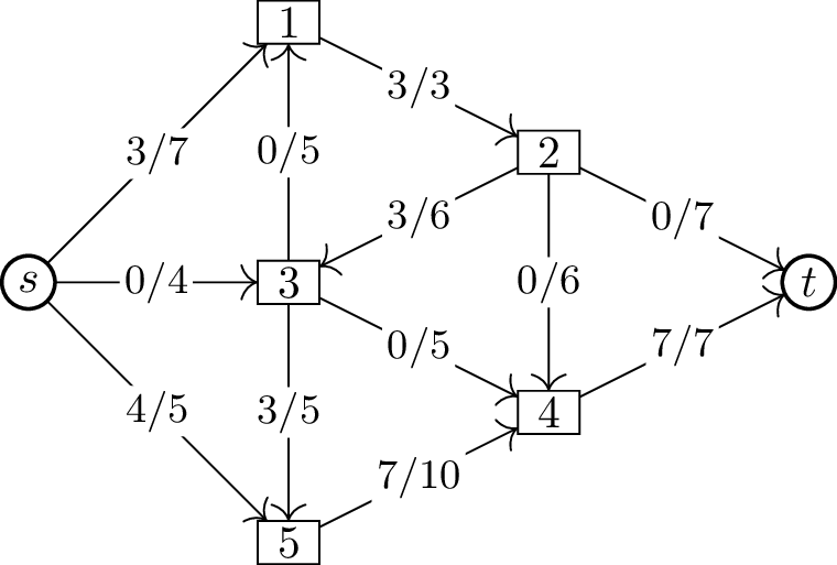
The diagram below gives a residual network for a network flow
problem.
Use the residual network to reconstruct the original network,
determining the arcs it has and their capacities.
Find the feasible flow which produces this residual
network.
Find a network cut whose capacity is equal to the value of the
flow.
Give an example showing that even if the capacities in a network
are all integers, it’s possible to have a maximum flow \(f\) such that not every value \(f(x,y)\) is an integer. (All we’ve proved
in this chapter is that the Ford–Fulkerson algorithm will never find
such a maximum flow.)
Prove that if \(f\) and \(g\) are two feasible flows, then the flow
\(h = \frac{f+g}{2}\) (that is, the
flow \(h\) with \(h(x,y) = \frac{f(x,y) + g(x,y)}{2}\) for
all arcs \((x,y)\)) is also a feasible
flow, and if \(f\) and \(g\) are both maximum flows, then so is
\(g\).
To prove the vertex version of Menger’s theorem using maximum
flows, we have to get a bit creative. In this practice problem, that’s
your job!
Given a directed graph \(D\) with
two vertices \(s\) and \(t\), not adjacent to each other, construct
a network \(N\) with integer capacities
and the following properties:
Given a \(k\)-vertex \(s-t\) cut in \(D\), we can find a network cut in \(N\) with capacity \(k\).
Given an integer flow in \(N\)
with value \(k\), we can find a set of
\(k\) internally-disjoint \(s-t\) paths in \(D\).
(If \(D\) has \(n\) vertices and \(m\) arcs, then it’s possible to construct
\(N\) so that it has \(2n-2\) vertices and \(m+n-2\) arcs.)
Prove that by being very clever about our choice of paths, it is
possible to find any maximum flow at the “greedy” stage of the
Ford–Fulkerson algorithm, without needing to use the residual network or
any backward arcs.
(This fact is not very useful in practice, since knowing the right
paths to use requires knowing the desired maximum flow in
advance.)
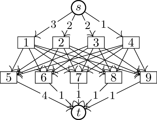
Find an integer flow in the network below. (The arcs whose
capacities are not marked should all be assumed to have capacity \(1\).)
Find a bipartite graph with bipartition \((A,B) = (\{1,2,3,4\}, \{5,6,7,8,9\})\) and
degree sequence \[(\deg(1), \deg(2), \dots,
\deg(9)) = (3,2,2,1,4,1,1,1,1).\]
Explain the connection between parts (a) and (b), and how the
network could be modified to find a bipartite graph with a different
bipartition and degree sequence.
In Chapter 17, we defined a \(2\)-factor in a graph \(G\) to be a \(2\)-regular spanning subgraph of \(G\).
Explain how to use the Ford–Fulkerson algorithm to solve the
following problem: given a graph \(G\),
either find a \(2\)-factor in \(G\), or determine that no \(2\)-factor exists.