I have to write about map coloring at some point in this textbook;
there’s no way around it. The map coloring problem is not only the
reason graph coloring was invented; it’s also a big part of the story
behind the invention of graph theory as a coherent discipline. That’s
also why there’s more history in this chapter of the textbook than in
most other chapters.
I don’t usually spend a whole lecture on map coloring when teaching a
course on graph theory, because there’s not enough time. I think going
up to just Theorem 24.4 is a reasonable minimum: it is a
good way to see how the properties of planar graphs we already know can
be applied, and it’s a nice application of coloring graphs greedily. The
proof of Theorem 24.5 I’ve included is a bit shorter than
the usual one, specifically in case you’ve decided to spend a bit more
time on the topic of map coloring, but not too much time. (As a side
note, the edge contraction in the proof has a particularly nice
representation if we are coloring a map, not a graph: then, we just
erase the borders region \(x\) has with
\(y_i\) and \(y_j\).)
The last two sections cover two special topics that are less
frequently seen in graph theory courses, but which I think are very
interesting. (I think it’s fascinating how—for the second time in our
study of planar graphs!—finding a Hamilton cycle can help us solve a
seemingly unrelated problem.) Heawood’s empire coloring problem is a
good example of how we can arrive at new mathematical questions by
examining the assumptions in our simplified models.
In addition to the previous chapters in this book, this chapter
heavily relies on Chapter 19
(naturally). On the other hand, the section on the use of Hamilton
cycles in coloring maps will not ask you to know much more from
Chapter 17 than the definition of a
Hamilton cycle.
Coloring maps
In Chapter 1, we visited Switzerland;
let us return there.
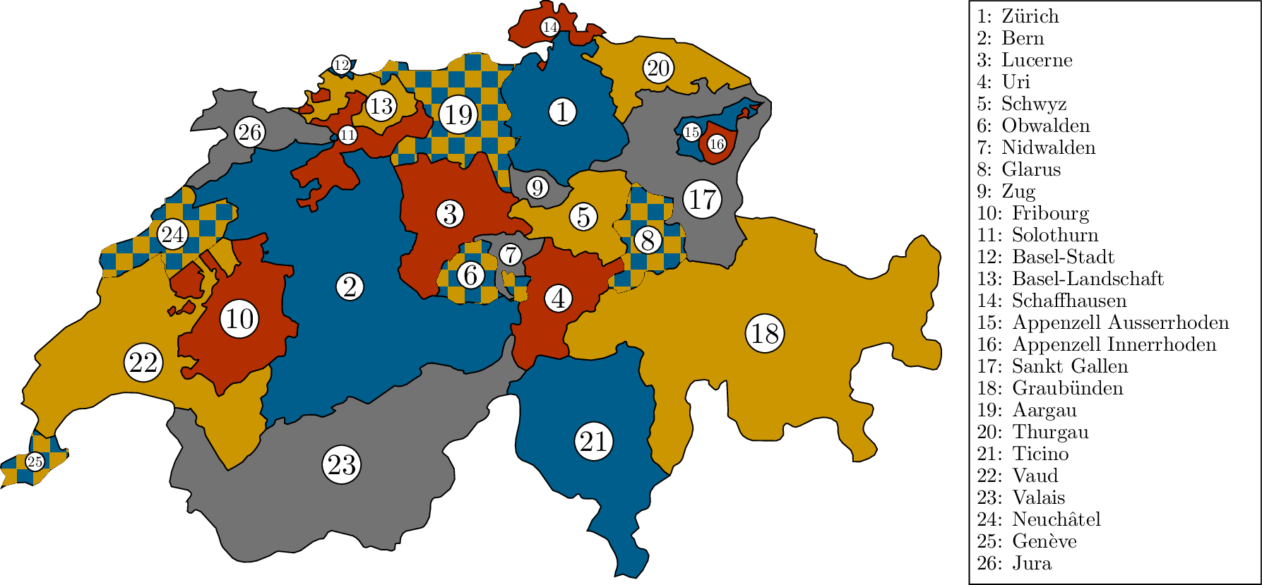
Figure 24.1 shows a map of
the cantons of Switzerland. To make the borders between cantons easy to
see, we give them different colors. We are willing to reuse colors, but
we would like two cantons to have different colors when they share a
border. (It would be fine for two cantons to have the same color if they
only share a corner; this situation is rarely found in maps.) How many
different colors do we need to color Switzerland—and is there a number
of colors that would be enough to color any map, no matter how
complicated?
Let the graph of adjacencies of a map be the graph
whose vertices are the regions we must color, with an edge between
vertices that share a border. Then what we are looking for is a (proper)
coloring of the graph of adjacencies: we’ve arrived back at the the
graph coloring problem studied in Chapter 19! Historically, in the
middle of the 19th century, this was the first graph coloring
problem studied. Graph theory had yet to be codified as a discipline at
the time, though some problems were studied individually which are now
the domain of graph theory. The book Four Colors Suffice by
Robin J. Wilson [107]
gives a history of the problem, and is also the source for most of my
historical claims in this chapter.
Why are we only looking at the map coloring problem now? The reason
is that for maps with reasonable, well-behaved regions, the graph of
adjacencies is planar. We can show this by the same argument we used to
prove Proposition 23.2 that the dual
graph of a plane embedding is planar. In fact, we can think of the graph
of adjacencies as the dual of a plane embedding whose edges are exactly
the borders drawn in the map. (We add vertices to give these edges
suitable endpoints; aside from a few edge cases, vertices are mostly
only necessary where three borders meet.)
I said “maps with reasonable, well-behaved regions” because the real
world is messy, and not all actual maps translate to planar graphs as
neatly. In fact, Switzerland already provides an example of this: its
cantons are not what I would call reasonable and well-behaved!
What properties do the Swiss cantons have
that the faces of a plane embedding shouldn’t?
They’re often not connected regions! Four
cantons have multiple pieces separated by another canton: Obwalden (6),
Fribourg (10), Solothurn (11), and Vaud (22).
In fact, we can prove that the graph of adjacencies between Swiss
cantons is not a planar graph. This follows from Kuratowski’s theorem
(Theorem 22.7). It’s enough to
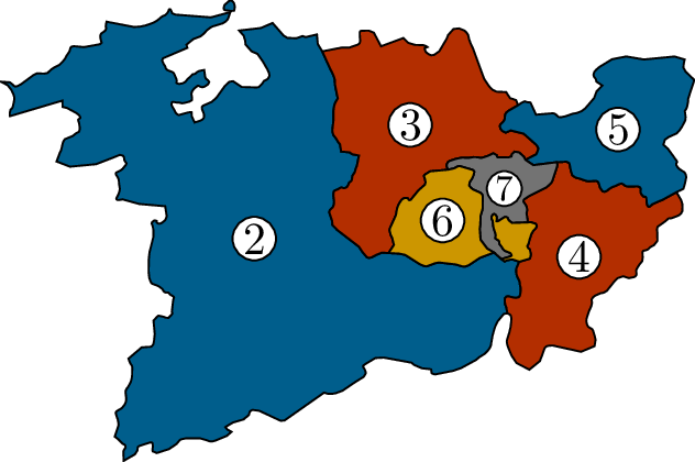
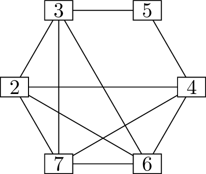
look at the cantons shown in Figure 24.2(a): because canton 6
(Obwalden) has two pieces, there are a few more borders between these
than would be possible in a reasonable map. The graph of adjacencies
between these \(6\) cantons contains a
subdivision of the complete graph \(K_5\), which is shown in Figure 24.2(b): \(9\) of the \(10\) edges between cantons \(\{2, 3, 4, 6, 7\}\) are present directly,
and instead of the edge \(\{3,4\}\)
there are edges \(\{3,5\}\) and \(\{5,4\}\) through \(5\), an extra vertex. (Edge \(\{5,7\}\) is also present in the graph, but
is not shown in Figure 24.2(b) because it is not part
of the subdivision.) Since the subgraph in Figure 24.2(b) is not planar, the
entire graph of adjacencies between Swiss cantons cannot be planar,
either.
A map of a few Swiss cantonsA subdivision of \(K_5\) in
Switzerland
Why Switzerland is not planar
This is an extremely practical example of a misbehaving map; it is
also possible to give another example that is extremely theoretical. Hud
Hudson showed [58] that
if we allow fractal regions with a finite area and infinite perimeter
(considering them to share a border if both regions get arbitrarily
close to that border), then even connected regions can touch in
extremely non-planar ways. There is no limit to the number of colors
that might be necessary to color such a fractal map.
From now on, we will assume that our maps are reasonable and
well-behaved: that the borders between regions obey the same
restrictions as edges in a planar graph (there are no fractal borders)
and that the objects we are coloring are nothing more than the connected
regions separated by those borders (there are no regions with multiple
pieces). With these caveats, the problem of coloring maps is exactly
equivalent to the problem of coloring planar graphs.
The four color theorem
What could stop us from coloring a map with \(k\) colors, for some integer \(k\)? The most straightforward kind of
obstacle is a set of \(k\) regions
among which any two are adjacent: a \(k\)-vertex clique in the graph we are
coloring. It’s possible to draw a map with four regions that all touch;
this is the simplest possible example of a map which requires four
colors.
Is it possible to draw a map with \(5\) regions that all touch?
No, because the graph of adjacencies would
be \(K_5\), which is not a planar
graph.
Does this prove that four colors are
enough to color any map?
No! It is possible to have a graph with no
\(5\)-vertex clique which is still not
\(4\)-colorable.
If you’ve been reading this book carefully and in order, Chapter 19 should already have
prepared you for the idea that the chromatic number \(\chi(G)\) and the clique number \(\omega(G)\) are very different. Forgetting
this is one of the most common mistakes people make when they first
think about coloring planar graphs.
From a pedagogical point of view, I can’t help but think that it’s a
shame that the following theorem really is true:
Theorem 24.1 (Four color theorem). If \(G\) is a planar graph, then \(\chi(G) \le 4\).
The road to proving this theorem has been a long one. The
mathematical question of whether four colors are enough to color any map
was first asked by Francis Guthrie in 1852. Later in the 19th
century, it received a great deal of mathematical attention, which came
with multiple incorrect solutions to the problem.
Some incorrect solutions were the sort of careless error that
confuses the chromatic number with the clique number. I assume that even
at the time, there were also many attempts to disprove the theorem, from
people who drew a very complicated map and could not find a way to color
it with four colors; there are still such attempts. (At the same time,
there was very persuasive experimental evidence for the four color
theorem: every real-world and imaginary map that was tried could in fact
be colored with four colors.)
There were also more notable attempts. Later on in this chapter, I
will mention two attempts at proving the four color theorem that were
eventually found to be false, but contributed a lot to graph theory,
even so. Alfred Kempe’s approach had a subtle error, but it was still
enough to give a proof of the weaker bound in Theorem 24.5, and the ideas in Kempe’s proof
have since been used to solve other problems about graph coloring. And I
suspect that Peter Tait’s use of Hamilton cycles to try to color maps
was one of the big reasons why 19th century mathematicians
continued to study Hamilton cycles, before practical uses of them were
found!
Eventually, a proof of the four color theorem was found, but even
that was controversial. Kenneth Appel and Wolfgang Haken, in a long
effort from 1972 to 1976, found a proof that relied on using a computer
to verify 1936 different configurations [4], [5]. How can any number of
finite cases be used to prove a theorem about the infinite variety of
possible maps? The idea, simplified, is that any possible map would be
guaranteed to contain one of the “reducible configurations” that Appel
and Haken found. The configurations were not just substructures that
could be colored: they could be replaced by smaller ones without hurting
colorability, which allows for a proof by induction on the number of
regions in the map.
A proof so long that it needed a computer to verify was
controversial. Wouldn’t it be invalidated by a single bug in the
program? This was the fear at first, but by now, it’s been nearly 50
years, and we can be a bit more confident, for a few reasons:
A 1997 proof by Robertson, Sanders, Seymour, and Thomas, while
still a computer-based proof, used fewer configurations and a simpler
approach to reductions [90].
In 2005, Georges Gonthier formalized the entire proof in the Coq
proof assistant [38].
Though the proof is still checked by computer in this case, it does not
rely on rules specific to map coloring, only on formal logic, so we can
be more confident in the computer.
It’s been nearly 50 years! If there were something incurably
wrong, surely we’d have discovered it by now.
Even if we believe the computer, there is still a reason why we might
want a short, human-readable proof (which still has not been found).
Such a proof would certainly contain new ideas that we can apply to
solve other, more difficult problems! This is not to say that the
computer-based proofs have no such insights; the whole approach of
reducible configurations, refined several times, is mathematically
interesting. But checking a large number of cases by computer does not
tell us whether there is some underlying simple reason why all those
cases would work.
You might have guessed by now that I will not show you a proof of the
four color theorem in this chapter. We will, however, look at the
arguments involved in proving two weaker bounds.
Greedy coloring
The greedy coloring algorithm goes through the vertices and gives
each one a color not already used on its neighbors. This algorithm is
guaranteed to find a coloring of the graph, but the number of colors
used depends on the order in which we color the vertices. The best thing
we can say about the greedy algorithm in general is that if a graph
\(G\) has maximum degree \(\Delta(G)\), it will never use more than
\(\Delta(G)+1\) colors.
Does give us any kind of universal upper
bound for planar graphs?
No: the maximum degree of a planar graph
can be arbitrarily high. For example, the star graph \(S_n\) is a tree with \(n-1\) leaf vertices adjacent to one central
vertex; it is planar (like all trees) but has maximum degree \(n-1\).
For planar graphs, it is possible to use some of the theory we’ve
already developed to order the vertices more intelligently. The
beginning is a bound on the minimum degree of a planar graph: though
planar graphs can have vertices of very large degree, this cannot be
true of every vertex.
Lemma 24.2. Every planar graph \(G\) has minimum degree \(\delta(G) \le 5\).
Proof. This is true for every planar graph with at most
\(6\) vertices because at that point,
you can’t have any degrees bigger than \(5\).
For planar graphs with \(n \ge 3\)
vertices and \(m\) edges, Theorem 22.2 tells us that \(m \le 3n-6\). However, if every vertex had
degree \(6\) or more, then we would
have \(m \ge \frac12(6n) = 3n\) by the
handshake lemma (Lemma 4.1), and we cannot
have \(3n \le 3n-6\). Therefore not all
vertices have degree \(6\) or more:
there must be a vertex with degree \(5\) or less. ◻
An alternate way to phrase the proof would be to look at the average
degree of a vertex, rather than the total number of edges.
What is the average degree of a graph with
\(n\) vertices and \(m \le 3n-6\) edges, and how does this help
us?
It is given by \(\frac{2m}{n} \le \frac{2(3n-6)}{n}\), which
simplifies to \(6 - \frac{12}{n}\).
Since \(6 - \frac{12}{n} < 6\), the
average degree is always less than \(6\). Not all vertices can be above average,
so there must be a vertex of degree less than \(6\).
It is convenient to have a vertex of small degree, because we can
leave it to be colored last: even if the worst should happen and all its
neighbors have different colors, we will still be able to pick a color
for it. For example, if we have \(6\)
colors available, and we leave a vertex of degree \(5\) until the end, it will always be
possible to give it a color.
If \(\delta(G)
\le 5\), is that enough to know that \(\chi(G) \le 6\): that \(G\) is \(6\)-colorable?
No! For example, we could start with \(K_{100}\) and add a new vertex of degree
\(5\) (or degree \(0\)). That low-degree vertex can be left
until the end, but we’ll still need \(100\) colors to color \(K_{100}\).
In the case of a planar graph, however, we know more. If we remove a
vertex of minimum degree, what we’re left with is a smaller planar
graph, and Lemma 24.2 also applies to that
smaller planar graph. That graph, too, has a vertex of degree \(5\) or less, which is enough to give us a
proof by induction.
Lemma 24.3. Every \(n\)-vertex planar graph \(G\) has a vertex ordering \(x_1, x_2, \dots, x_n\) in which each vertex
is adjacent to at most \(5\) of the
vertices that come before it.
Proof. We will prove this by induction on \(n\). When \(n \le
6\), any vertex ordering will do.
Assume that the lemma is true for all \((n-1)\)-vertex planar graphs, and let \(G\) be an \(n\)-vertex planar graph. By Lemma 24.2, \(\delta(G) \le 5\); let \(x\) be a vertex with \(\deg_G(x) \le 5\).
Apply the induction hypothesis to find a vertex ordering \(x_1, x_2, \dots, x_{n-1}\) of \(G-x\). We can extend it to a vertex
ordering of \(G\) by setting \(x_n = x\). For all \(i \le n-1\), \(x_i\) has fewer than \(5\) neighbors among \(\{x_1, x_2, \dots, x_{i-1}\}\) by the
induction hypothesis. Meanwhile, \(x_n\) has fewer than \(5\) neighbors among \(\{x_1, x_2, \dots, x_{n-1}\}\) because it
has fewer than \(5\) neighbors
total.
By induction, we can find such a vertex ordering for all \(n\). ◻
Using this lemma, we can prove our first bound on the chromatic
number of arbitrary planar graphs!
Theorem 24.4. If \(G\) is a planar graph, then \(\chi(G) \le 6\).
Proof. Let \(x_1, x_2, \dots,
x_n\) be the vertex ordering given by Lemma 24.3, and let \(C\) be a set of \(6\) colors. For \(i=1, 2, \dots, n\) in that order, give
\(x_i\) an arbitrary color in \(C\) not already used on its neighbors.
Why is this possible? Because \(x_i\) only has \(5\) neighbors in the set \(\{x_1, x_2, \dots, x_{i-1}\}\), and these
are the only vertices already given a color when we get to \(x_i\). So at most \(5\) of the \(6\) colors in \(C\) have been used on the neighbors of
\(x_i\), and there is still a color
left to choose.
When we’re done, the coloring we get is proper, because we never give
a vertex a color used on an adjacent vertex. For every edge \(x_i x_j\), where \(i < j\), we already knew the color of
\(x_i\) when we got to \(x_j\), and we made sure that \(x_j\) would be given a different
color. ◻
Five colors
Suppose we want to go one step further, and prove that \(\chi(G) \le 5\) for all planar graphs \(G\).
What would go wrong if we tried the
methods in the previous section to prove this?
We would encounter planar graphs with
minimum degree \(5\). Here, we cannot
leave any vertex for last and forget about it; its neighbors might end
up with \(5\) different colors, and we
would have no color left to use on the last vertex.
Are there, in fact, any planar graphs with
minimum degree \(5\)?
Yes, and we’ve seen them already: the
skeleton graph of the icosahedron is one example.
We can still try to find an recursive algorithm for \(5\)-coloring planar graphs: given a planar
graph \(G\) and a vertex \(x\) of minimum degree, we \(5\)-color \(G-x\) and then complete the result to a
coloring of \(G\). However, if \(\deg_G(x) = 5\), we will need to do one of
two things:
Before we color \(G-x\), modify
it somehow to ensure that we’ll be able to put back \(x\) and give it a color.
After we color \(G-x\), modify
the coloring somehow to ensure that we’ll be able to put back \(x\) and give it a color.
Historically, the first proofs of Theorem 24.5 used the
second approach, modifying the coloring using subgraphs called Kempe
chains; this idea is similar to the recoloring strategy we used in the
proof of Vizing’s theorem (Theorem 20.6).
Kempe chains are named after Alfred Kempe, who used the idea in 1879 in
a proposed proof of the four color theorem. In 1890, Percy Heawood found
a subtle error in Kempe’s proof, but the argument via Kempe chains was
still the first argument showing that five colors are always enough to
color any map.
We will instead take the first approach, which is a shorter and more
direct argument. This proof is due to Paul Kainen [60] and is a much later invention.
Theorem 24.5. If \(G\) is a planar graph, then \(\chi(G) \le 5\).
Proof. We induct on \(n\),
the number of vertices of \(G\). (This
will be a strong induction, because sometimes we’ll need to go back from
\(n\) to \(n-2\), not just \(n-1\).) If \(n
\le 5\), then of course \(G\)
has a coloring with at most \(5\)
colors; this gives us our base cases.
Now assume that all planar graphs with fewer than \(n\) vertices have colorings with at most
\(5\) colors, and let \(G\) be an \(n\)-vertex planar graph. By Lemma 24.2, \(G\) has a vertex \(x\) of degree at most \(5\).
If in fact \(\deg(x) \le 4\), then
we have lucked out. By induction, \(G-x\) has a coloring with at most \(5\) colors. In that coloring, the neighbors
of \(G\) use at most \(4\) of the colors, because there are at
most \(4\) of them, so we can give
\(x\) a color none of them use. The
result is a coloring of \(G\).
If \(\deg(x) = 5\), let \(y_1, y_2, y_3, y_4, y_5\) be the neighbors
of \(x\). The first thing we observe is
that it’s not possible for all of the edges between \(y_1, \dots, y_5\) to be present in \(G\).
Why not?
Then they’d form a copy of \(K_5\) (a copy of \(K_6\), in fact, when taken together with
\(x\)), which we know is not planar;
but \(G\) is a planar graph.
So let \(y_i\) and \(y_j\) be two of \(x\)’s neighbors that are not adjacent in
\(G\). (We’ll see why this matters
soon!) Construct a graph \(H\) in the
following steps:
Delete all edges from \(x\)
except edges \(xy_i\) and \(xy_j\).
Contract edges \(xy_i\) and
\(xy_j\), obtaining a new vertex \(z\).
Deleting and contracting edges preserves planarity, so \(H\) is a planar graph on \(n-2\) vertices. By our induction
hypothesis, \(H\) has a \(5\)-coloring. Extend this \(5\)-coloring to \(G-x\) by giving \(y_i\) and \(y_j\) the color of \(z\).
Why is this a proper coloring?
Every neighbor of \(y_i\) or \(y_j\) in \(G -
x\) was a neighbor of \(z\) in
\(H\), so it had a different color from
the color used on \(z\). Therefore in
\(G-x\), it has a different color from
the color used on \(y_i\) and \(y_j\). This is all that needs to be
checked; for all other edges, both endpoints have the same color in
\(G-x\) and in \(H\).
What would have gone wrong if \(y_i\) and \(y_j\) were adjacent?
Then both endpoints of the edge \(y_i y_j\) would have the same color, so the
coloring of \(G-x\) would not be
proper.
Now we have a \(5\)-coloring of
\(G-x\) in which only \(4\) different colors are used on the
neighbors of \(x\), because two of them
(\(y_i\) and \(y_j\)) have the same color. Once again,
this lets us give \(x\) a color not
used on any of its neighbors and obtain a coloring of \(G\).
This proves the induction step, and so the theorem is true for planar
graphs with any number of vertices. ◻
Hamilton cycles
In 1880, Peter Tait proposed several solutions of his own to the map
coloring problem. At the time, Kempe’s 1879 proof was generally
accepted; Tait merely felt that the proof was too complicated, and
wanted a simpler one. None of Tait’s solutions worked out in the sense
of giving an alternative proof, but several of them were successful in
giving alternate avenues of attack on the problem.
Earlier, I mentioned that the graph of adjacencies of a map is the
dual of a plane embedding whose edges are exactly the borders drawn in
the map. However, we did not really consider this plane embedding as an
object of study in its own right. Tait was the first to do so, and was
able to get remarkably close to a proof of the four color theorem in
this way.
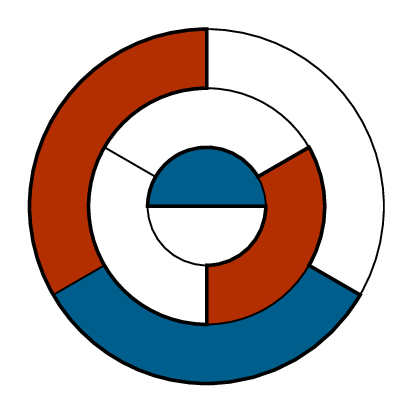
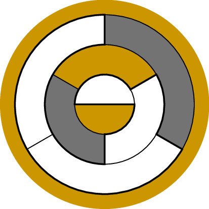
Tait began by finding a Hamilton cycle in this plane embedding; for
an example, consider the Hamilton cycle in Figure 24.3(a). The Hamilton cycle divides the
plane embedding into two parts, an inside and an outside. Tait’s
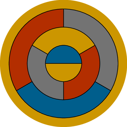
strategy was to color those two parts separately (see Figure 24.3(b) and Figure 24.3(c)) then combine the colorings,
as shown in Figure 24.3(d).
A Hamilton cycleColor the insideColor the outsideThe final result
Using a Hamilton cycle in the borders of a map to \(4\)-color it
Why would this help? Well, Tait noticed that the inside and the
outside of the cycle can each be colored with just two colors: four
total! In fact, the graph of adjacencies on either side of the Hamilton
cycle is a tree, and as we know (Proposition 13.3), all
trees are bipartite, or in other words \(2\)-colorable.
To see this, let \(H\) (for “half”)
be the graph of adjacencies on just one side of the Hamilton cycle. Each
edge in \(H\) exists due to a border in
the plane embedding where we drew the Hamilton cycle; both endpoints of
that border lie on the cycle, because it’s a Hamilton cycle. If a border
is drawn between two points on a closed loop, it cuts that loop in half,
separating the two parts of the side it’s drawn on. Back in \(H\), that makes the edge we were looking at
a bridge. A connected graph in which every edge is a bridge is a
tree.
Why is this not a proof of the four color
theorem?
The missing detail is that we don’t yet
have a reason to believe that the Hamilton cycle we are relying on
exists!
In fact, it’s pretty easy to draw a map in which we can’t draw a
Hamilton cycle along the borders. (Switzerland is an example: here, the
borders aren’t even connected!) Tait was aware of this, but still had
hope to do it in all the worst cases, which would be enough to prove the
four color theorem.
What are the worst cases? The phrase “worst case” is one you should
generally watch out for in your proofs: if you’re not careful, it can
lead to unjustified assumptions. To properly use it, we should first
explain how every other case is simpler than some “worst” case.
That’s exactly what we can do here. Suppose we are trying to color an
arbitrary planar graph \(G\). If there
is any edge \(xy\) such that adding
\(xy\) to \(G\) produces another planar graph \(G+xy\), then we might as well add it! Every
coloring of \(G+xy\) is also a coloring
of \(G\), with the extra restriction
that \(x\) and \(y\) cannot be given the same color. And if
we think we have a rule for coloring all planar graphs, that rule should
be able to handle \(G+xy\) just as well
as \(G\).
This means that it’s enough to consider only maximal planar graphs,
which cannot gain any new edge and still be planar. By Proposition 22.4, these
are exactly the graphs whose plane embeddings are always
triangulations.
What do we know about the dual of a
triangulation?
The condition that each face has length
\(3\) turns into a condition that each
vertex has degree \(3\). They are \(3\)-regular graphs!
(In fact, not all \(3\)-regular
planar graphs are the duals of triangulations; the graph must also be
\(3\)-connected, but we won’t
learn what that means until Chapter 26.)
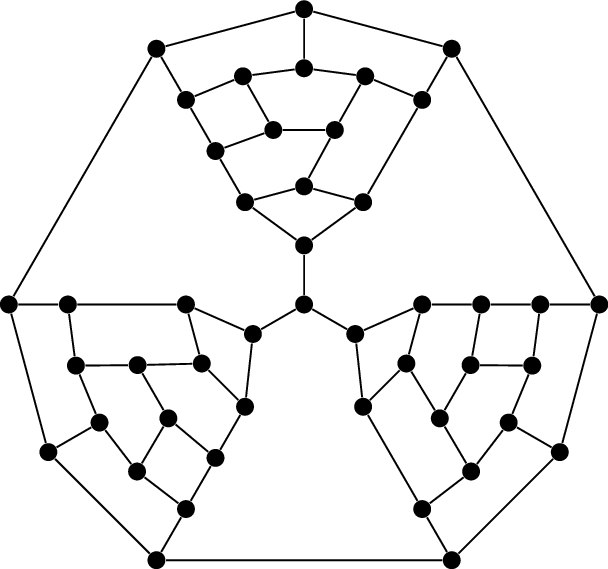
Tait’s conjecture was that the dual graph of every triangulation is
Hamiltonian. If this were true, it would imply the four color theorem,
by the strategy we pursued in Figure 24.3(a). This
seemed to be a viable strategy for a long time; it was not until 1946
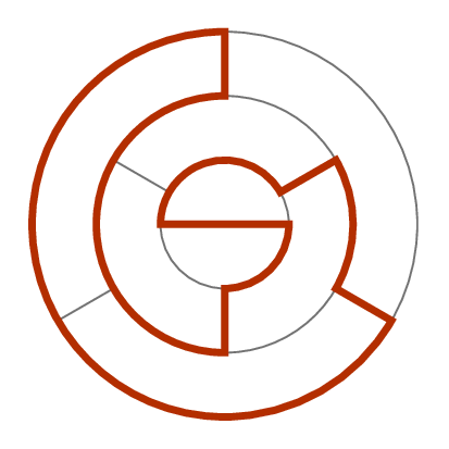
that Tutte found a counterexample [98]. That counterexample is shown in Figure 24.4 and is known as the Tutte
graph. (Here, the planar graph which cannot be colored using Tait’s
strategy is the dual of the Tutte graph; that is, we wish to color the
faces in Figure 24.4. By the four color theorem, of
course, this is still possible—just not via finding a Hamilton
cycle.)
The Tutte graph
Coloring empires
In 1890, along with finding the flaw in Kempe’s attempt at the four
color theorem, Heawood asked [54]: what about maps like the map of
Switzerland? That is, what about maps where a single country can have
multiple disconnected parts, which must be given the same color?
If we don’t put some kind of restriction on this ability, then there
is no limit to the number of colors we might need.
Why not?
For example, give each country a tiny
exclave in the middle of each other country’s territory. Now this
prevents those two countries from sharing a color, so every country will
need a different color.
Heawood’s approach was to express the problem in terms of the maximum
number of parts a single country can have. Unfortunately, he did not
come up with a clever name for such divided countries. This omission was
corrected by Martin Gardner when writing about Heawood’s work much
later [36]; Gardner
proposed the term \(M\)-pire
for an empire whose territory consists of at most \(M\) disconnected pieces.
Let’s begin by looking at the case \(M=2\). (This more or less describes
Switzerland; though some Swiss cantons have more than \(2\) pieces, this does not contribute any
additional adjacencies.)
Proposition 24.6. A map of \(2\)-pires can always be colored using at
most \(12\) colors so that two \(2\)-pires which share a border (in at least
one of their territories) receive different colors.
Proof. We can model a map of \(2\)-pires in two ways:
With a graph (call it \(H\)) in
which vertices are connected regions, and an edge exists whenever two
regions share a border. Let there be \(n\) regions; then (as we’ve already seen)
this graph is planar and has at most \(3n-6\) edges.
With a graph (call it \(G\)) in
which vertices are the empires, and an edge exists between two vertices
if some territory belonging to one empire borders some territory
belonging to the other empire. This is the graph we actually want to
color.
In \(G\), there are also at most
\(3n-6\) edges! That’s because every
edge in \(G\) must come from an edge in
\(H\) (a border shared is a border
shared in either representation) but every edge in \(H\) corresponds to at most one edge in
\(G\) (a shared border only belongs to
two empires).
Is it possible for \(G\) to have fewer edges than \(H\)?
Yes: whenever one empire touches two of
another empire’s regions, that is represented by two edges in \(H\), but only one edge in \(G\).
What can we say about the number of
vertices in \(G\)?
It could be as high as \(n\) (if every \(2\)-pire is actually an ordinary country),
but cannot go below \(n/2\): with at
most \(2\) regions per empire, it takes
at least \(n/2\) empires to reach \(n\) regions.
The average degree in \(G\) is \(\frac{2|E(G)|}{|V(G)|}\) by the handshake
lemma, or at most \(\frac{3n-6}{n/2} = 12 -
\frac{24}{n}\). In particular, it is less than \(12\), so \(\delta(G) < 12\).
What’s more, if we delete a vertex \(x\) from \(G\), then the remaining graph \(G-x\) is also the graph of adjacencies of
some map of \(2\)-pires: just erase
empire \(x\) from the map! This means
that \(\delta(G-x) < 12\), by the
same argument, and in general, every subgraph of \(G\) will have a vertex of degree less than
\(12\).
We can now color \(G\) by the same
greedy argument as we used to prove Theorem 24.4, using
\(12\) colors instead of \(6\). Leaving a low-degree vertex until the
end guarantees that one of \(12\)
colors will be available for it, since its neighbors have at most \(11\) different colors. ◻
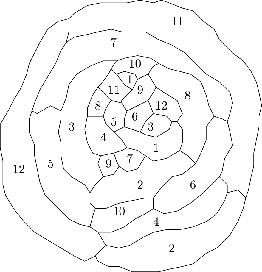
Heawood’s map of 12 pairwise adjacent empires
Theorem 24.4 was considerably more pessimistic
than the truth: it says that \(\chi(G) \le
6\) for all planar graphs \(G\),
but actually, it is also true that \(\chi(G)
\le 4\). Does Proposition 24.6 have a
similar flaw?
No: it turns out that it is the best possible bound! Figure 24.5 shows a map drawn by
Heawood. Here, there are \(12\) empires
(labeled \(1\) through \(12\)), and any two of them share a border!
For this map, it is impossible to use fewer than \(12\) colors, because all empires must have
different colors; therefore there cannot be a general result better than
Proposition 24.6.
Heawood gave an argument for the general case of \(M\)-pires, as well.
What upper bound does the same argument
give for a map of \(M\)-pires?
An upper bound of \(6M\) colors: with \(n\) regions, there are still at most \(3n-6\) edges (less than \(3n\)) but the number of \(M\)-pires is at most \(n/M\), so the average degree is less than
\(\frac{2(3n)}{n/M} = 6M\).
However, he was unable to find a map to show that this was the best
upper bound when \(M \ge 3\), and left
this as a conjecture. This conjecture was resolved almost a century
later, when Brad Jackson and Gerhard Ringel showed how to construct such
maps for all \(M\ge 2\)[59].
Practice problems
Find a \(4\)-coloring of the
faces of an icosahedron.
Prove that \(3\) faces are not
enough to color the faces of an icosahedron.
Even though Switzerland’s graph of adjacencies is not planar, it
is still \(4\)-colorable! Find such a
\(4\)-coloring. (You may prefer to
refer to the diagram in Figure 1.2(b) all
the way back in the first chapter instead of a map of
Switzerland.)
The mathematician August Ferdinand Möbius is perhaps best known
for his mathematical study of the Möbius strip: the surface formed by
taking a strip of paper and joining the two ends with a half-twist, so
that the two sides of the paper are turned into one side. In regards to
coloring maps, his contribution was to show that \(5\) connected regions on a map cannot all
share borders with each other; an early form of proving that \(K_5\) is not planar.
Ironically, when drawing a map on a Möbius strip rather than in the
plane, it is possible to have \(5\)
regions all border each other. How can this be done?
As a follow-up, see if you can do it for \(6\) regions.
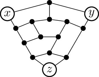
The Tutte graph shown in Figure 24.4 is
made up of three subgraphs isomorphic to the one shown below, plus a
central vertex. The three vertices labeled \(x\), \(y\), and \(z\) in the diagram are used to connect the
three subgraphs together: each \(x\)-vertex is joined to a \(y\)-vertex in a different subgraph to
connect the three cyclically, and the three \(z\)-vertices are all joined to the center
vertex of the Tutte graph.
Show (by casework) that the graph above has no \(x-y\) Hamilton path. (It does have \(x-z\) and \(y-z\) Hamilton paths, which you may feel
free to find, though they won’t be useful for the next step.)
Use part (a) to show that the Tutte graph has no Hamilton
cycle.
Here are several coloring problems for the union of two graphs.
The graphs may share vertices and even edges; their union is a graph
containing every vertex and every edge present in at least one of the
graphs.
The union of two planar graphs is \(12\)-colorable. Explain why this is a
special case of Proposition 24.6.
By imitating the proof of Proposition 24.6, prove
that the union of two trees is always \(4\)-colorable.
Prove that the union of two bipartite graphs is always \(4\)-colorable.
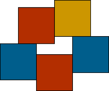
The faraway and fictional continent of Kvadrat is divided into
many countries, all in the shape of \(1\times
1\) squares. The squares are not necessarily aligned to a grid,
and might have unclaimed land between them (which does not need to be
given a color). One possible map is shown below:
Can all possible maps of Kvadrat be colored using only three colors,
or is there an example of such a map which requires four
colors?
The faraway and fictional country of Heibai is divided into
cantons, just like Switzerland, but its map has a curious property: at
every point where several borders meet, the total number of borders that
converge there is even. (The United States has just one point of this
type: the point where Arizona, Colorado, New Mexico, and Utah come
together.)
Prove that it’s possible to color the cantons of Heibai with just two
colors so that two cantons that share a border are always colored
differently. (Two cantons that only share a point may have the same
color.)
Let \(G\) be a planar graph that
has been partially \(5\)-colored: there
is a set \(W \subseteq V(G)\) such that
every vertex \(x \in W\) has already
been given a color \(f(x) \in
\{1,2,3,4,5\}\), which cannot be changed.
Prove that if the distance between any two vertices in \(W\) is at least \(4\), then this partial coloring can be
completed to a \(5\)-coloring of \(G\). (This result was proved by Michael
Albertson in 1998 [1].)