Bonus Chapter: Crossing Numbers

The purpose of this bonus chapter

As an extension of studying planar graphs and their plane embeddings, it is natural to study drawings of general graphs in the plane with few crossings. Even though I did not include this content in the textbook for reasons of time and space, it would fit quite well at some point after Chapter 22 or perhaps Chapter 23. (However, the probabilistic machinery used to prove the crossing number inequality is a bit more advanced than what I use in the textbook.)

As I started writing this bonus chapter, a mini-theme developed: the theme of incorrect proofs. It appears that proofs of bounds on crossing numbers can be quite tricky, and easy to make subtle mistakes in! We all learn best from mistakes—ideally, other people’s mistakes—so I have included some opportunities for you to test whether you can spot the error in a proof.

For most of this document, I have consulted the original sources I am citing, but when writing the section on complete graphs, I referenced the book Crossing Numbers of Graphs by Marcus Schaefer [6]. This is also a good place to read more about crossing numbers, though it is written at a more advanced level than this bonus chapter.

Not-quite-planar graphs

What are the non-planar graphs that are as close as possible to being planar?

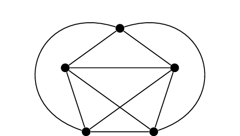
Probably the most reasonable answer is: the graphs \(K_5\) and \(K_{3,3}\). By Kuratowski’s theorem (Theorem 22.7), every non-planar graph contains a subdivision of one of these graphs, so in some sense, any graph is at least as non-planar as \(K_5\) and \(K_{3,3}\). We cannot, of course, draw \(K_5\) or \(K_{3,3}\) without crossing edges, but we can draw them with just one crossing edge. How? You could probably figure it out yourself, but I have given one way to do it in Figure 1(a) (for \(K_5\)) and in Figure 1(b) (for \(K_{3,3}\)).

If we delete one of the crossing edges from these diagrams, we are left with a planar graph.¹ On the other hand, there are also graphs which are one edge away from being planar, but cannot be drawn in the plane without many crossings!

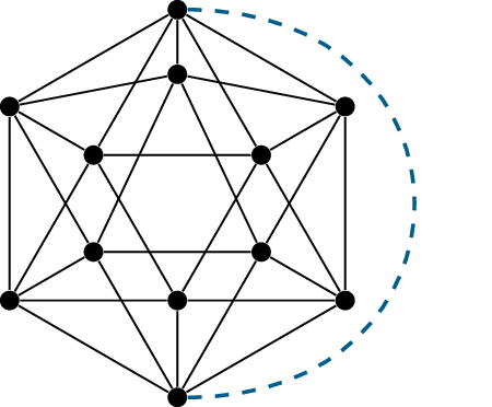
To find one such graph, consider what happens when we start with the skeleton graph of the icosahedron and add an extra edge between two opposite vertices, as shown in Figure 2(a). All the faces of the icosahedron are triangles, so the graph was already a maximal planar graph; with the addition of the extra edge, it stops being planar.

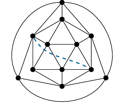
If we need to draw this graph in the plane, how many crossings do we need? Well, Figure 2(b) shows a solution with three crossings; it is obtained by starting with a plane embedding of the icosahedral graph, and then drawing the extra edge to cross as few of the existing edge as possible.

You might worry that there were other ways to attempt to draw the graph that would have resulted in fewer crossings. Let me give you some reassurances!

First, there’s no better plane embedding of the icosahedral graph which we could have started with, in which the endpoints of the extra edge are somehow closer together. Of course, we can wiggle around the vertices and edges in various ways, and we can change which face is the outer face, but we’ll still be looking at more or less the same picture. In particular, in any plane embedding, by Proposition 22.4, all faces must be triangles. By Euler’s formula (Theorem 21.4), there must be \(20\) triangular faces. But there are only \(20\) cycles of length \(3\) in the graph, so it is these cycles that must bound each face of whatever plane embedding you pick.

Second, there’s no way to draw the extra edge that crosses fewer than three existing edges. The number of crossings forced by the extra edge is determined by the number of faces it must pass through: if the extra edge must pass through at least four faces, then it must cross their boundaries at least three times. A quick way to see that the extra edge must, indeed, pass through at least four faces is to use the distance-finding algorithm from Chapter 3.

Label the five faces whose boundary contains the top vertex with a \(0\): these can be reached without crossing any edge. Label their neighboring (and unlabeled) faces with a \(1\): these can be reached by crossing only one edge. Label their neighboring (and unlabeled) faces with a \(2\): these can be reached by crossing only two edges. We end by labeling the last five faces with a \(3\), showing that we must cross three edges at a minimum to reach them; these five faces are exactly the five faces whose boundary contains the bottom vertex.

What do you think?

Have I successfully given a proof that the graph in Figure 2 cannot be drawn in the plane with fewer than three crossings?

No; this proof still has a gap in it!

How do you know that the optimal drawing of this graph is obtained by starting from a plane embedding of the icosahedral graph? Perhaps we can draw that graph in a different way, with one or two crossings—but then add the extra edge in a way that generates fewer additional crossings, or maybe none at all!

One of the practice problems at the end gives a better way to approach this question, which does not leave such a gap.

The crossing number

Let’s generalize the ideas we’ve seen in these examples.

First, we should ask: when we talk about drawings of a graph in the plane in this bonus chapter, what sort of drawings are we considering?

Most of the setup can be inherited from Chapter 21, where we discussed plane embeddings of graphs for the first time. Of course, one thing has to change: we now allow edges to cross. However, we should still be careful about how they are allowed to cross.

• First of all, we should not allow an edge to pass through a vertex (except by starting and ending at one). Otherwise, it’s unclear how to count that intersection.

• Second, we should not allow three or more edges to cross at the same point. If we did, any graph could be drawn with just one crossings. (I leave the details to you, in practice problem 1.)

• Third, it will make our lives easier to assume that two edges incident to the same vertex \(x\) never cross. It’s easy to imagine drawings in which they do cross, but whenever this happens, we can always modify the drawing to eliminate the crossing.

  In particular, edges should not cross themselves!

With these caveats in mind for the definition that follows and the rest of the chapter, we say:

In this terminology, we’ve shown that \(\operatorname{cr}(K_5) = \operatorname{cr}(K_{3,3}) = 1\), and I’ve given you most of a proof that the graph in Figure 2 has crossing number \(3\).

If we trust that example, then it’s possible for a graph to be one edge away from planar, and still have a crossing number bigger than \(1\). What about the other way around: can every graph \(G\) with \(\operatorname{cr}(G)=1\) be made planar by deleting one edge?

Yes: simply take a drawing of \(G\) with only one crossing, and delete an edge \(e\) involved in the crossing! The resulting drawing is a plane embedding of \(G-e\).

If a graph \(G\) has crossing number \(\operatorname{cr}(G) = k\), then a proof that \(\operatorname{cr}(G) \le k\) can be very short: just draw a picture! To prove that \(\operatorname{cr}(G) \ge k\), we need to make an argument that applies to every embedding, and (as we’ve already seen by example) this can be very difficult. Just like the invariants discussed in Chapter 17, Chapter 18, and Chapter 19, computing the crossing number is a hard problem.

It’s even harder than that actually. If I asked you, “Is the complete graph \(K_n\) Hamiltonian?” or “What is the chromatic number of the complete bipartite graph \(K_{n,n}\)?” then you would have an immediate answer. Meanwhile, the crossing numbers of these graphs (in general, in terms of \(n\)) are still open questions!

The brick factory problem

We should start with the complete bipartite graph, because it is easier (but not easy!) and because it is historically the first crossing number to be studied in graph theory. The problem first appears in print in a 1955 article by Casimir Zarankiewicz [8], but its origin is attributed to Pál Turán, who had to deal with it in a practical situation.²

In 1944, Turán was working in a brick factory near Budapest. There were \(n\) kilns where the bricks are made and \(m\) storage yards where they were kept. (We do not know the exact numbers, so we have no choice but to deal in variables.) All the kilns were connected by rail to all the storage yards, forming a drawing of the complete graph \(K_{m,n}\) in the plane. Since \(m\) and \(n\) were both at least \(3\), the rails had to cross in some places.

The small trucks rolling on the rails had a great deal of trouble at the crossings; they would derail (both Turán and Zarankiewicz describe this as a regular occurrence, not an occasional one) and spill the bricks. Naturally, we want to minimize the crossings; but how can this be done? In other words; what is \(\operatorname{cr}(K_{m,n})\) as a function of \(m\) and \(n\)?

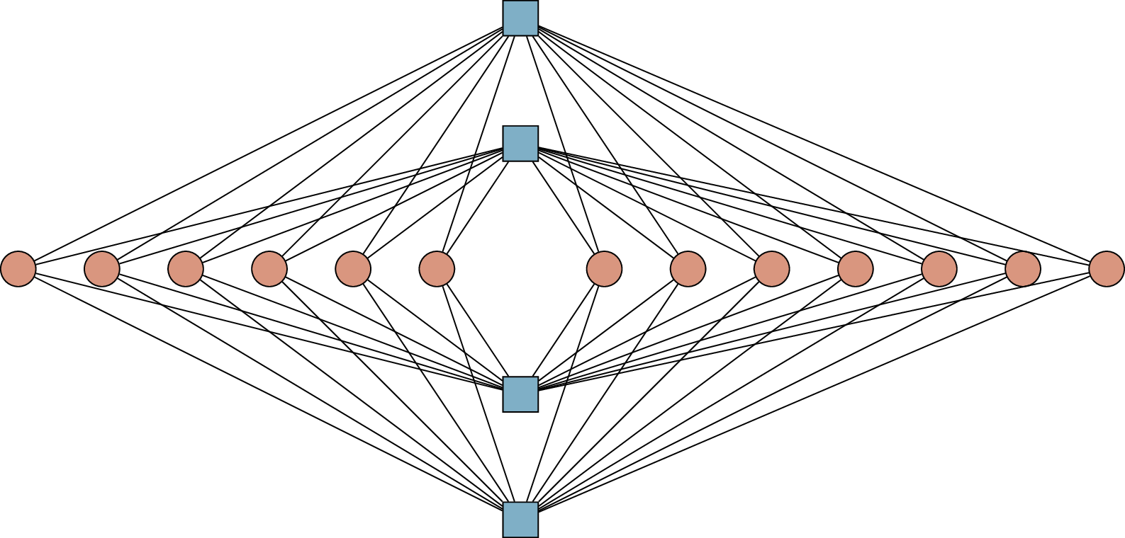
Zarankiewicz found, first of all, a general method to draw \(K_{m,n}\) in the plane without too many crossings. This is illustrated in Figure 3 on the example of \(K_{4,13}\). In general, to draw \(K_{m,n}\), the vertices on one side of the bipartition are placed along the \(y\)-axis, half above the \(x\)-axis and half below. The vertices on the other side of the bipartition are placed along the \(x\)-axis, half to the left of the \(y\)-axis and half to the right. When \(m\) and/or \(n\) are odd, the vertices cannot be split in half exactly, so we divide them as close to equally as possible.

In this construction, in order for two edges \(ab\) and \(a'b'\) (where \(a,a'\) are drawn on the \(y\)-axis and \(b,b'\) on the \(x\)-axis) to cross, several things have to happen. First of all, the two edges have to be drawn in the same quadrant: this happens if \(a\) and \(a'\) were sorted into the same half, and so were \(b\) and \(b'\). Second, if \(a\) is further from the origin than \(a'\), then \(b\) must be closer to the origin than \(b'\), and vice versa; among the four edges \(\{ab, ab', a'b, a'b'\}\), there is only one intersection.

This description is enough to give a formula for the number of crossings in the drawing we get. It takes a bit more work to obtain the simplest expression for the formula, which is generally accepted to be the following: \[\operatorname{cr}(K_{m,n}) \le \left\lfloor \vphantom{\frac12} \frac n2 \right\rfloor \left\lfloor \frac {n-1}2 \right\rfloor \left\lfloor \vphantom{\frac12}\frac m2 \right\rfloor \left\lfloor \frac {m-1}2 \right\rfloor.\] (This is an upper bound on \(\operatorname{cr}(K_{m,n})\), because it’s the number of crossings in only one possible drawing; there could be a better drawing!)

This construction is generally believed to give the least possible number of crossings. This is now called the Zarankiewicz conjecture³, but that’s not how Zarankiewicz thought of it. He thought that he found a proof of a matching lower bound, but it turned out to have a gap in it.

I do not bring this up to criticize Zarankiewicz. First of all, every mathematician has written many proofs with mistakes in them; it is a regrettable part of doing mathematics, and we just hope that someone finds the mistakes. Second, since 1955, nobody has been able to do better and find a correct proof. I bring this up because I am going to present Zarankiewicz’s proof to you, and make you figure out what is wrong with it.

The proof begins with a correct lemma, which gives a correct lower bound in the case \(m=3\). Pay careful attention to the proof of this lemma.

The intended proof of the general case that Zarankiewicz gave works very similarly, but with one key difference that makes it fail. Can you find it?

If you were paying attention, you should have been asking yourself this question all along, but:

Where is the mistake in this proof? What does the induction in Lemma 1 do right that the intended proof of the general case does wrong?

In the proof of Lemma 1, removing the vertices \(x\) and \(y\) is guaranteed to eliminate every crossing involving the edges \(1x, 1y, 1z\), \(2x, 2y, 2z\), \(3x, 3y, 3z\), so it eliminates the \(n-2\) “extra crossings” we got: the remaining \(\lfloor \frac{n-2}{2}\rfloor \lfloor \frac{n-3}{2}\rfloor\) crossings are different ones.

In the intended proof of the general case, for each pair \(\{y,z\}\), we found \(\lfloor \frac n2\rfloor \lfloor \frac{n-1}{2}\rfloor\) crossings between the edges out of \(x\), \(y\), and \(z\). However, if some of these crossings are between an edge out of \(y\) and an edge out of \(z\), then those crossings remain when we delete vertex \(x\). In that case, they are also counted among the \(\lfloor \frac n2\rfloor \lfloor \frac{n-1}{2}\rfloor \lfloor \frac{m-1}{2}\rfloor \lfloor \frac{m-2}{2}\rfloor\) crossings we get from the induction hypothesis, and overall they are double-counted.

If you did not spot the error, do not feel bad; it took eleven years after Zarankiewicz’s publication for it to be discovered!

The complete graph

An equally natural but trickier problem is determining \(\operatorname{cr}(K_n)\), as a function of \(n\). Here, too, we have a construction that we believe is optimal, but we cannot prove it…

…and actually, things are even more interesting than that. We have two constructions, which give the same upper bound in two completely separate ways. That seems like very good evidence that they are in fact the best construction, even though we have no proof. (We have yet to find a better construction, which is also good evidence!)

For both constructions, it helps to first think about what happens if we don’t try at all to find the best solution. Let’s draw \(K_n\) in the usual way, by placing the \(n\) vertices as points spaced around a circle. It’s tempting to space them evenly around a circle, but that violates our rules about drawings: we will usually get many points where three or more edges intersect. For example, if \(n\) is even, there would be \(n/2\) diameters intersecting at the center of the circle.

Instead, we can place the vertices at \(n\) points on a circle at random! For example, generate a uniformly random angle \(\theta \in [0,2\pi]\) for each vertex, and draw it at the point with coordinates \((\cos \theta, \sin\theta)\). It does not actually matter too much how we do it, as long as enough randomness is injected, because in a continuous world, it’s an incredible coincidence when three chords of a circle all pass through the same point.

Another common way to add randomness is to start with a diagram where some intersections might be bad, and randomly move every point by a very tiny amount; this also eliminates all triple intersections. Mathematicians call this a perturbation, and sometimes say that a diagram is in general position when all such unlikely coincidences are eliminated.

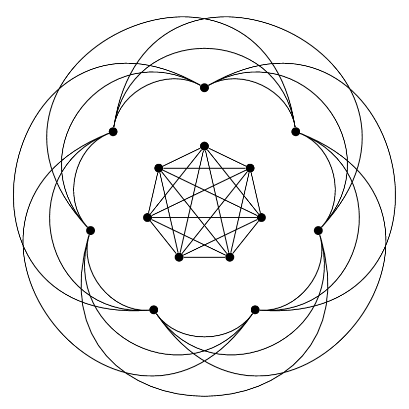
The same drawing can also be turned “inside out”, drawing every edge as a curve outside the circle rather than a chord inside the circle. The same crossings show up: two curved edges outside the circle intersect each other if and only if they would have intersected inside the circle as chords.

We are not especially excited to have two ways to draw \(K_n\) with \(\binom n4\) crossings, but we can use them both at once to draw \(K_{2n}\) efficiently.

First, draw a small copy of \(K_n\) with straight edges, and a larger copy of \(K_n\) around it with “inside out” curved edges, as shown in Figure 4(a) for \(n=7\). What’s missing? We still need to draw the edges between the two copies of \(K_n\).

This is the same as drawing \(K_{n,n}\); why can’t we just reuse the results from the previous section?

Unfortunately, we’re restricted in where we can place the vertices, and with this vertex placement, the Zarankiewicz construction cannot be used.

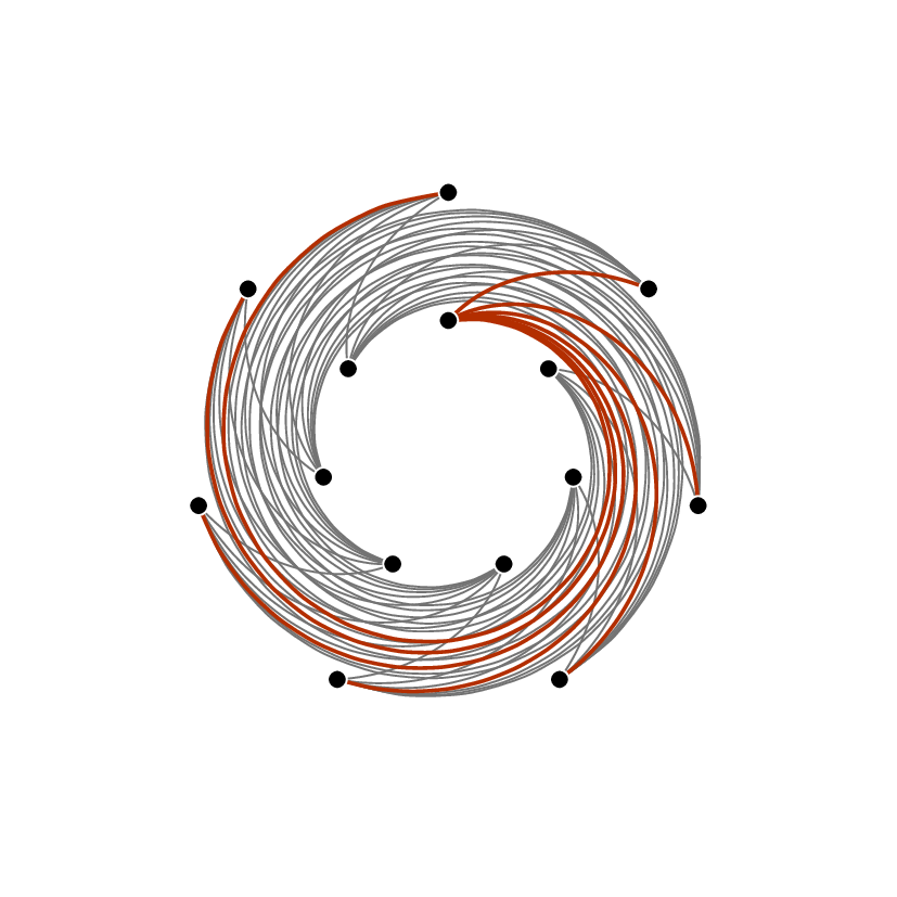
We will take an artistic approach and draw all edges as spirals going clockwise from inside to outside, as shown in Figure 4(b); the edges incident to the top inside vertex are highlighted in red, to make the pattern easier to see.

It may seem silly that, in particular, to go from an inside vertex to the very closest outside vertex, we have a spiral winding all the way around! This does not add additional crossings, though. If you imagine rotating the inner copy of \(K_7\) halfway, you can make all the spirals shorter (and some will reverse), without changing which spirals cross.

To count all the crossings in Figure 4(b), we will first count the total number of times that a spiral highlighted in red crosses a spiral which is shorter. (We’ll do it in general, for all \(n\).) Here, the reason why the spirals wind around as much as they do becomes apparent: I did it to make the counting more natural.

Number the positions of the vertices clockwise around the circle by \(0, 1, 2, \dots, n\), with positions \(0\) and \(n\) being the same. The highlighted spirals are exactly the spirals which start in inside position \(0\). If a highlighted spiral from inside position \(0\) to outside position \(k\) crosses a shorter spiral, then the shorter spiral must go from inside position \(i\) to outside position \(j\), where \(i < j < k\). There are \(\binom n3\) ways to choose \(i\), \(j\), and \(k\) such that \(1 \le i < j < k \le n\), so there are \(\binom n3\) crossings between a highlighted spiral and a shorter spiral.

We’re now on the finish line! Multiply by \(n\) to account for the \(n\) different inside vertices where the highlighted spirals could have started. Add the \(2\binom n4\) crossings within the two copies of \(K_7\), and we learn that this construction has \[2\binom n4 + n \binom n3 = \frac14 n(n-1)^2(n-2)\] crossings in total.

Why do I insist on only counting crossings where the highlighted spiral is longer?

Otherwise, we will count each crossing twice, once from the perspective of each spiral.

This construction only works for \(K_{2n}\), but it can be modified slightly for an odd number of vertices. If each crossing involves two edges with four different endpoints, then the average vertex is involved in a \(4/n\) fraction of the crossings: \((n-1)^2(n-2)\) of them. But the construction is extremely symmetrical: every vertex should be involved in the same number of crossings! (The only tricky part of seeing that is turning the diagram “inside out” to see that the inside vertices are no different from the outside ones.) So by deleting any vertex we like, we get a drawing of \(K_{2n-1}\) with \[\frac14 n(n-1)^2(n-2) - (n-1)^2(n-2) = \frac14 (n-1)^2(n-2)(n-4)\] crossings.

We have obtained a proof of the following theorem, due to Richard Guy [3]:

Another way to express the upper bound of Theorem 3, unifying the even and odd cases, is \[\operatorname{cr}(K_n) \le \frac14 \left\lfloor \vphantom{\frac12} \frac n2 \right\rfloor \left\lfloor \frac{n-1}{2}\right\rfloor \left\lfloor \frac{n-2}{2}\right\rfloor \left\lfloor \frac{n-3}{2}\right\rfloor.\]

I mentioned two constructions. The second, due to Frank Harary and Anthony Hill [4], is conceptually more natural, but harder to analyze. Starting with the drawing of \(K_n\) in Lemma 2, Harary and Hill ask: what if we turn only some of the edges inside out, drawing them as curves outside the circle? I will leave the story of what happens next to you, in the last practice problem.

The crossing number inequality

A graph with \(n \ge 3\) vertices and \(3n-5\) edges has too many edges to be planar, by Theorem 22.2, so its crossing number must be at least \(1\). We can prove a generalization of this, if the graph exceeds the upper limit of \(3n-6\) edges by more than \(1\).

If \(m\) is large, however, then Lemma 4 is very weak. The graph \(K_{100,100}\) has \(200\) vertices and \(10\,000\) edges, so Lemma 4 tells us that it has at least \(9\,400\) crossings. That’s over nine thousand, but much less than \(\lfloor \frac{100}{2}\rfloor \lfloor \frac{99}{2}\rfloor\lfloor \frac{100}{2}\rfloor\lfloor \frac{99}{2}\rfloor = 6\,002\,500\): the number of crossings that we’d get if the Zarankiewicz conjecture were true.

Can we do better? Let’s try.

Of course, Lemma 5 is not always better than Lemma 4, but it is better when \(m\) is much larger than \(n\). For example, it tells us that \(\operatorname{cr}(K_{100,100}) \ge 37\,600\), so we’ve made a tiny bit of progress in the direction of what we believe to be true.

What just happened here? This style of argument resembles a story of Baron Munchausen [5]. The Baron is riding a horse, when he finds himself in a swamp, sinking deeper and deeper by the moment. What does he do? He pulls himself free by his own hair: “Gripping my noble steed with both knees, I seized my pigtail with my free hand and pulled myself and my horse out of the bog.”

In our case, too, it seems like we proved Lemma 5 using nothing more but the weaker tool of Lemma 4. How is this possible?

Well, Lemma 4 is only bad when the number of edges far exceeds the number of vertices. When the graph is more sparse, it is not such a bad bound! So we switch from looking at \(G\) to looking at \(H\), a subgraph of \(G\). We do not know which subgraph \(H\) is best to look at, and in such a case, we take the resort of the probabilistic graph theorist: we pick \(H\) at random.

We can keep going, though. The argument carried to its logical conclusion is a theorem first shown by Ajtai, Chvátal, Newborn, and Szemerédi [2], though the probabilistic argument and the better bound it implies is attributed to Chazelle, Sharir, and Welzl.⁴

They did not prove the result below, which is missing an important qualifier. I will present a proof of the theorem without the qualifier; the proof will, accordingly, have an error. As you read, try to tell me: where did I cheat?

Before asking the big question and trying to figure out what’s wrong with this proof, let’s ask a little question: where did \(\frac{4n}{m}\) come from?

A little bit of calculus can get it for us. If we had used a variable probability \(p\), then we would have arrived at the inequality \[p^4 \operatorname{cr}(G) - p^2 m + 3p n \ge 0 \implies \operatorname{cr}(G) \ge \frac{pm - 3n}{p^3}.\] We would like the largest possible lower bound, so we must choose the value of \(p\) that makes this quantity as large as possible. Setting the derivative equal to zero and solving, we get…

…well, we get \(p = \frac{4.5n}{m}\), actually. But the resulting inequality is \(\frac{4m^3}{243n^2}\), which is not much better, and a bit messier. For practical reasons, \(p = \frac{4n}{m}\) and a \(64\) in the denominator is good enough.

There’s only one problem with the theorem we get: it’s clearly, painfully wrong on simple examples.

Let \(G\) be the cycle graph \(C_n\). What does Theorem 6 tell us about \(G\)?

Since \(C_n\) has \(n\) vertices and \(n\) edges, the bound in Theorem 6 simplifies to \(\operatorname{cr}(C_n) \ge n/64\).

Why is that so bad?

Well, \(C_n\) is a planar graph: draw it as a regular \(n\)-sided polygon, and there are no crossings. So the lower bound \(\operatorname{cr}(C_n) \ge n/64\) is wrong for all \(n\): it is always positive. For large cycles like \(C_{64\,000}\) the bound is not just wrong but very wrong.

The mistake in the proof is one which can often be easy to make in proofs by the probabilistic method, like this one. However, if you’ve never written or read such a proof before, you may not be on guard against it.

We are only allowed to say “keep a vertex with probability \(\frac{4n}{m}\)” if \(\frac{4n}{m}\) really is a probability: if it is between \(0\) and \(1\). So the condition we must add is that \(m \ge 4n\). This is not a hardship, since we plan to use the theorem on graphs with many more edges than that.

Now let’s state the theorem correctly. (The theorem is also often called the “crossing lemma”, but it’s also one of the biggest results in this bonus chapter, so I had to make it a theorem.)

For example, if we return once again to the case of \(K_{100,100}\), we get a much better lower bound: any drawing of this graph must contain at least \(390\,625\) crossings.

Theorem 7 also tells us something more general: that the drawings of \(K_n\) and \(K_{n,n}\) which we believe to have the fewest crossings are at the very least only off by a constant. If we simplify, the theorem tells us that \(\operatorname{cr}(K_n) \ge \frac{n(n-1)^3}{512}\) and that \(\operatorname{cr}(K_{n,n}) \ge \frac{n^4}{256}\). Both of these are degree-\(4\) polynomials in \(n\). Our upper bounds are also degree-\(4\) polynomials in \(n\) (ignoring floors and ceilings): we can now confirm that at least we’ve gotten that part right!

Practice problems

1. Suppose that we relax the conditions in our drawings, and allow any number of edges to cross at the same point.

   Prove that now, every graph can be drawn in the plane with at most one crossing point. (It’s enough to prove that this can be done for \(K_n\) for every value of \(n\).)

2. Prove that for any graph \(G\), if \(H\) is a subdivision of \(G\), then the crossing numbers of \(G\) and \(H\) are equal.

3. One way to deal with the graph in Figure 2 is to prove that if two “ordinary” edges of the graph are deleted, but the extra edge is kept, the result can never be planar.

   1. I verified this fact by a brute-force search in Mathematica, but try to convince yourself informally by finding many subdivisions of \(K_{3,3}\) using the extra edge, so that it’s impossible to destroy all of them by removing only one or two ordinary edges.

   2. Explain why it follows from this fact that the graph has crossing number at least \(3\).

4. Prove that \(\operatorname{cr}(K_6) = 3\).

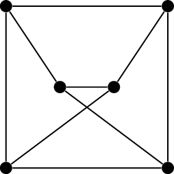
5. Prove that \(\operatorname{cr}(Q_4) \ge 4\). (It is known that \(\operatorname{cr}(Q_4) = 8\), but I do not know if that is easy to prove.)

6. Use Theorem 22.6 to help you prove that the Petersen graph has crossing number \(2\).

7. 1. In a drawing of \(K_n\) in the plane, every copy of \(K_6\) is drawn with at least \(\operatorname{cr}(K_6) = 3\) crossings. This does not mean that there are \(3\binom n6\) crossings total, because many of them are counted multiple times.

      If we correct for the double-counting, what lower bound on \(\operatorname{cr}(K_n)\) do we get?

   2. In a drawing of \(K_n\) in the plane, every copy of \(K_{n-1}\) is drawn with at lest \(\operatorname{cr}(K_{n-1})\) crossings. This does not mean that there are \(n \cdot \operatorname{cr}(K_{n-1})\) crossings total, because many of them are counted multiple times.

      If we correct for the double-counting, what inequality between \(\operatorname{cr}(K_{n-1})\) and \(\operatorname{cr}(K_n)\) do we get?

   3. Use induction and the inequality in part (b) to obtain another lower bound on \(\operatorname{cr}(K_n)\).

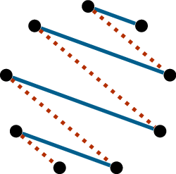
8. In this problem, you will investigate the ideas behind the Harary–Hill construction for drawing \(K_n\) with few crossings. As a reminder, we position the \(n\) vertices around a circle, and draw each edge either as a chord of the circle or as a curve outside the circle.

   It would be too complicated to make the decision for each edge, so we group them together into \(n\) matchings: if \(V(K_n) = \{1,2,\dots,n\}\), then the \(k\)^th matching \(M_k\) consists of the edges \(xy\) with \(x+y \equiv k \pmod n\).

   1. Prove that if \(n\) is odd, then \(|E(M_k)| = \frac{n-1}{2}\) for all \(k\). This is impossible when \(n\) is even; what happens then?

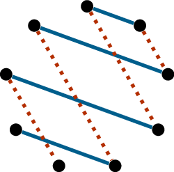
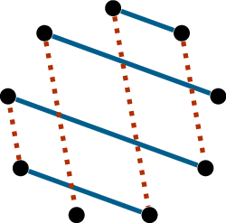
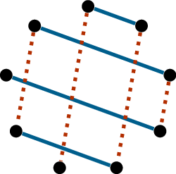
   2. If \(M_i\) and \(M_j\) are both drawn on the same side of the circle, how many crossings are there between them, in terms of \(i\), \(j\), and \(n\)? The four distinct cases when \(n=9\) are shown below:

      

   3. To avoid cases where the answer to (b) is large, if we split the \(n\) matchings into half inside and half outside, how should we do it?

   4. Verify that the total number of crossings in this case matches the bound in Theorem 3.

Footnotes

1. This also follows from Kuratowski’s theorem. For example, if an edge is deleted from \(K_5\), the resulting graph cannot contain a subdivision of \(K_5\), since it does not have enough edges, nor a subdivision of \(K_{3,3}\), since it does not have enough vertices. Thus it must be planar!↩︎

2. Later, in 1977, Pál Turan gave his own account of the story, as part of a welcoming note [7] in the first issue of the Journal of Graph Theory.↩︎

3. It is not called Zarankiewicz’s conjecture, because nobody knows how to pronounce the “…cz’s” ending.↩︎

4. “The proof we now present arose from e-mail conversations between Bernard Chazelle, Micha Sharir and Emo Welzl,” write Martin Aigner and Günter Ziegler in Proofs from the Book [1].↩︎

References

1. Aigner, M., K. H. Hofmann, and G. M. Ziegler. 2014. Proofs from THE BOOK. Mathematics and Statistics. Springer Berlin Heidelberg.
2. Ajtai, Miklós, Václav Chvátal, Monroe Newborn, and Endre Szemerédi. 1982. “Crossing-Free Subgraphs.” North-Holland Mathematics Studies 60: 9–12. https://doi.org/10.1016/S0304-0208(08)73484-4.
3. Guy, Richard. 1972. “Crossing Numbers of Graphs.” In Graph Theory and Applications, edited by Y. Alavi, D. R. Lick, and A. T. White, 111–24. Berlin, Heidelberg: Springer Berlin Heidelberg. https://doi.org/10.1007/BFb0067363.
4. Harary, Frank, and Anthony Hill. 1963. “On the Number of Crossings in a Complete Graph.” Proceedings of the Edinburgh Mathematical Society 13 (4): 333–38. https://doi.org/10.1017/S0013091500025645.
5. Raspe, R. E. et al. 1903. The Wonderful Adventures of Baron Munchausen [by R.E. Raspe and Others] Adapted for Children by d. Hayman. https://books.google.com/books?id=6fjfTok6LM8C.
6. Schaefer, Marcus. 2018. Crossing Numbers of Graphs. CRC Press. https://doi.org/10.1201/9781315152394.
7. Turán, Pál. 1977. “A Note of Welcome.” Journal of Graph Theory 1: 7–9. https://doi.org/10.1002/jgt.3190010105.
8. Zarankiewicz, Casimir. 1955. “On a Problem of P. Turan Concerning Graphs.” Fundamenta Mathematicae 41: 137–45. https://doi.org/10.4064/fm-41-1-137-145.