This chapter presents three different approaches by which we can
(sometimes or always) determine whether a graph is planar.
The first is Theorem 22.2, which is also very useful as a
property of planar graphs: in Chapter 24, you will see
how. It is especially important if you are not yet a very experienced
mathematician to remember that this is very much not an if-and-only-if
condition; do not use it in the wrong direction!
The second is Kuratowski’s theorem and Wagner’s theorem, which I
group together, because they are very similar. As a planarity test,
looking for minors is more powerful than looking for subdivisions, but
minors are harder to understand—when teaching this material, I have
often skipped Wagner’s theorem for that reason. I include it here
because in Chapter 24, it will be
useful for us to know about edge contractions.
The third is the method of overlap graphs developed by Tutte. This is
not as commonly studied, but I don’t know why, because it’s great. Any
other equally systematic approach to planarity testing is much harder to
learn.
Counting edges in planar
graphs
In the previous chapter, we proved two tools that help us count
vertices, edges, and faces in a plane embedding: the face length formula
(Lemma 21.3)
and Euler’s formula (Theorem 21.4). We will now
use these to prove a limit on the number of edges that a planar graph
with \(n\) vertices can have.
For this, we will have to restrict our attention to simple graphs
only, even though both results above apply to multigraphs as well.
Otherwise, there is no possible bound we can prove!
Why can a planar multigraph with \(n\) vertices have arbitrarily many
edges?
Starting from an arbitrary plane
embedding, we can draw in any number of loops at a vertex without
crossings—imagine a flower with the loops as the petals, and the vertex
at the center. If there is more than one vertex, we can also replace an
edge by any number of parallel copies without affecting planarity.
We can engage in some meta-reasoning and ask: if our argument is to
work for simple planar graphs, but not for planar multigraphs, what must
it be doing? What sort of situations can only appear in the plane
embedding of a multigraph?
Well, once again, we’re back to the way that we can draw loops and
parallel edges in a plane embedding. These are not unusual: they are the
way we draw loops and parallel edges by default in a diagram of a
multigraph. From the point of view of the counting tools we have,
though, what makes them special is that they are boundaries of a face of
length \(1\) (in the case of a loop) or
\(2\) (in the case of two parallel
edges).
Do loops and parallel edges have to be
drawn as faces of length \(1\) or \(2\)?
No: at least in the case of some graphs,
it’s possible to draw the graph so that some part of it is inside the
loop, or between the two parallel edges. (An example appears in the
first practice problem at the end of the previous chapter.)
Are there any simple graphs with faces of
those lengths?
Just one: a graph with two vertices and a
single edge between them has a plane embedding in which the outer face
has length \(2\).
The following short lemma is the property we use to distinguish
simple graphs from multigraphs. (From now on until we conclude our
discussion of the number of edges in a planar graph, I will assume all
graphs are simple.)
Lemma 22.1. In a plane embedding of a simple
graph with at least \(2\) edges, every
face has length at least \(3\).
Proof. If the plane embedding has multiple faces, then each
face needs to be separated from the other faces somehow; its boundary
must contain a closed curve, which corresponds to a cycle in the graph.
The graph is simple, so a cycle in it must contain at least \(3\) edges.
If the plane embedding has only one face, then every edge of the
graph must contribute \(2\) to the
length of that face. There are at least \(2\) edges, so the face has length at
least \(4\). ◻
When we feed Lemma 22.1
into the tools we have from the previous chapter and let it cook, we
obtain the following theorem.
Theorem 22.2. For all planar graphs with \(n \ge 3\) vertices and \(m\) edges, \(m
\le 3n-6\).
Proof. Choose a plane embedding of a graph with \(n \ge 3\) vertices and \(m\) edges to work with for the rest of the
proof. Let \(r\) be the number of faces
it has; by Lemma 22.1, each face has length at
least \(3\), so the sum of the lengths
of all the faces is at least \(3r\).
What if Lemma 22.1 does not apply, because
\(m<2\)?
Then \(m\le
3n-6\) automatically, because \(3n-6
\ge 3(3)-6 = 3\).
By the face length formula, the sum of the lengths of all the faces
is also equal to \(2m\), giving us the
inequality \(2m \ge 3r\). We would like
to combine this inequality with Euler’s formula: \(n - m + r - k = 1\). We do not know \(k\), the number of connected components,
but it’s certainly at least \(1\), so
we get a second inequality: \(n - m + r \ge
2\).
Our goal in this proof is to establish a relationship between \(m\) and \(n\) (though it can be interesting to look
at the other two pairs of variables, too), so we should eliminate \(r\). We solve for \(r\) in the inequality \(2m \ge 3r\) (getting \(r \le \frac23m\)) and in Euler’s formula
(getting \(r \ge m - n + 2\)). Putting
them together, we get \[m - n + 2 \le
\frac23m\] which we can rearrange to \(\frac13m \le n-2\), or \(m \le 3n-6\). ◻
What would we learn if we eliminated \(m\) instead of eliminating \(r\)?
From \(m \le n +
r - 2\) and \(m \ge \frac 32r\),
then \(n + r - 2 \ge \frac 32r\), or
\(r \le 2n - 4\). This tells us the
maximum number of faces in an \(n\)-vertex planar graph.
This chapter is called “Planarity testing”, and Theorem 22.2 is our first planarity test: it lets
us immediately conclude that some graphs are not planar! Here is an
example:
Proposition 22.3. The complete graph \(K_5\) is not planar.
Proof. We count: \(K_5\)
has \(n=5\) vertices and \(m=10\) edges. Since \(3n - 6 = 9\), which is less than \(m\), the conclusion of Theorem 22.2 does not hold. Therefore the
hypotheses do not hold either, so \(K_5\) is not a planar graph. ◻
If an \(n\)-vertex graph has \(3n-6\) or fewer edges, can we conclude from
Theorem 22.2 that it is planar?
No: the theorem gives a necessary
condition for planarity, but not a sufficient one. For example, take
\(K_5\) and add \(95\) isolated vertices, and you’ll get a
\(100\)-vertex graph with only \(10\) edges which is not planar.
Triangulations
Whenever we prove an inequality, a natural question to ask is: what
can we say about the cases where equality holds? What kind of planar
graphs have \(m = 3n-6\)?
To draw conclusions about such graphs, we should look back at our
proof, and look at every place where an inequality appeared. This is an
extremely useful idea not just in graph theory, but in other areas of
math!
We wrote Euler’s formula as an inequality: \(n - m + r \ge 2\). If it were the case that
\(n - m + r > 2\), we would conclude
that \(m < 3n-6\).
So if a planar graph with \(n\ge3\)
vertices satisfies \(m = 3n-6\), then
\(n - m + r\) must be equal to \(2\), meaning that the graph is
connected.
The inequality \(m \le 3n-6\)
combines Euler’s formula with the inequality \(2m \ge 3r\). If we had started with the
strict inequality \(2m > 3r\), we
would have arrived at the strict inequality \(m < 3n-6\), instead.
So if a planar graph with \(n\ge 3\)
vertices satisfies \(m = 3n-6\), it
must satisfy \(2m = 3r\).
The inequality \(2m \ge 3r\)
itself comes from another inequality, but one we only stated in words:
Lemma 22.1, which says that every face
has length at least \(3\). (For all
faces \(F\), \(\operatorname{len}(F) \ge 3\).)
So if a planar graph with \(n\ge 3\)
vertices satisfies \(m = 3n-6\), then
every face must have length exactly \(3\), and this must be true in every plane
embedding of the planar graph.
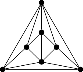
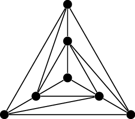
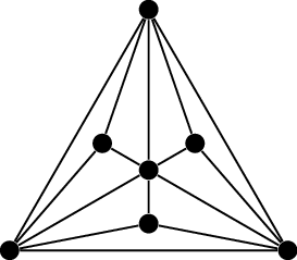
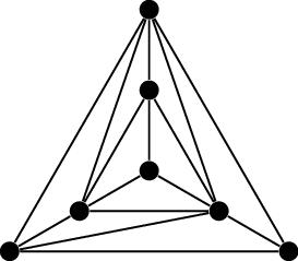
Now that we’ve understood these extremal examples, we give them a
name, based on the fact that all of their faces are (in some sense)
triangles. We call a plane embedding of a connected graph in which all
faces have length \(3\) a
triangulation. For each \(n\), there are many \(n\)-vertex triangulations; see Figure 22.1 for some examples when \(n=7\). (These are all the \(7\)-vertex possibilities, up to isomorphism
of the planar graph. I know this because I first looked up sequence
A000109 [79] in the Online Encyclopedia of Integer Sequences to confirm there are \(5\) of them,
then searched the House of Graphs[20] to find out what they are.)
Triangulations with \(7\)
vertices
To be clear, “triangulation” is a term for the plane embedding, not
for the planar graph. How do we refer to the planar graph, then? The
corresponding notion is a maximal planar graph: a planar graph
that stops being planar if any edge (that it does not already have) is
added to it. But to avoid sneaking in a claim that has not been
justified, we need the following proposition.
Proposition 22.4. For a planar graph \(G\) with \(n \ge
3\) vertices, the following are equivalent:
\(G\) has \(3n-6\) edges.
Every plane embedding of \(G\) is a triangulation.
\(G\) is a maximal planar
graph.
Proof. We have already proven that \(\text{(i)} \iff \text{(ii)}\). \(G\) has exactly \(3n-6\) edges if and only if every
inequality in the proof of Theorem 22.2 is an
equality: if and only if every face has length exactly \(3\). This has to happen regardless of the
plane embedding we choose at the beginning of that proof, so it must be
true for every plane embedding.
Which other implication between (i), (ii),
and (iii) is easiest to show?
The implication \(\text{(i)} \implies \text{(iii)}\) also
follows from Theorem 22.2. If \(G\) has \(3n-6\) edges, and we add a new edge to
\(G\), then we get a graph with \(3n-5\) edges, so by the contrapositive of
Theorem 22.2, the new graph is not planar.
The part of Proposition 22.4
that we still need to prove is that (iii) also implies (i) and (ii). In
other words, there are no maximal planar graphs that “get stuck” before
reaching \(3n-6\) edges. We will show
that (iii) implies (ii), and we will do it by showing the
contrapositive: if \(G\) has an
embedding that’s not a triangulation, then \(G\) is not a maximal planar graph.
Our strategy has a short description: in a plane embedding of \(G\) that isn’t a triangulation, we find a
face \(F\) with \(\operatorname{len}(F) \ge 4\), and then we
add an edge between two vertices on the boundary of \(F\), drawing it inside \(F\). The reason this is not the entire
proof is that we have to make sure the edges do not already exist inside
\(F\).
In order for that to even be a problem, \(F\) must not be the only face, which means
that there is a cycle on the boundary of \(F\) separating it from the other faces.
This is either a cycle of length \(4\)
or more, or else a cycle of length \(3\) with some more vertices of \(F\) “inside” the cycle; in either case,
there are at least \(4\) vertices on
the boundary of \(F\).
If there are \(5\) or more vertices
on the boundary of \(F\), then they
cannot all be adjacent: \(G\) would
then contain a copy of \(K_5\), which
we know cannot be drawn in the plane. If there are only \(4\) vertices, and they are all adjacent,
then the plane embedding of \(G\) would
contain a plane embedding of \(K_4\) in
which \(F\) is a face. This is
impossible: by \(\text{(i)} \implies
\text{(ii)}\), every plane embedding of \(K_4\) is a triangulation, and cannot
contain a face like \(F\) of length
more than \(3\).
Does anything change if \(F\) is the outer face?
Not substantially; the outer face is
outside the cycles on its boundary, rather than inside them, but nothing
changes aside from that one word.
In all cases, at least two vertices \(x,y\) on the boundary of \(F\) are not already adjacent in \(G\). If we add edge \(xy\) to \(G\), the result is still planar, because
drawing a curve from \(x\) to \(y\) inside \(F\) gives a plane embedding of \(G+xy\). This completes the proof: it shows
that \(G\) is not a maximal planar
graph. ◻
Girth and planarity
Before we go on to necessary and sufficient conditions for planarity,
let’s try to squeeze a bit more power out of the approach used to prove
Theorem 22.2, because counting edges is a simpler
test than just about anything else we could try.
The most common scenario is when \(G\) is a bipartite planar graph. In this
case, the boundary of a face cannot be a cycle of length \(3\): by Theorem 13.1, bipartite graphs
cannot contain such cycles! This allows us to sharpen our
inequality.
What if the boundary of a face is not a
cycle?
In general, the length of the face is the
total length of its boundary walks, and in a bipartite graph, all closed
walks have even length.
If the minimum length of a face is \(4\), then we replace the inequality \(2m \ge 3r\) in the proof of Theorem 22.2 by the inequality \(2m \ge 4r\). As before, when we want an
upper bound on \(m\), we may assume
\(G\) is connected, which lets us apply
Euler’s formula: \(n - m + r = 2\).
Eliminating \(r\) and simplifying, we
conclude:
Theorem 22.5. For all planar bipartite graphs
with \(n\ge 3\) vertices and \(m\) edges, \(m
\le 2n-4\).
To appreciate the power of this approach, we can go back to
Proposition 21.1
from the previous chapter. At the time, we need a technical argument
that looked closely at the geometry of a plane embedding in order to
prove that \(K_{3,3}\) is not planar.
With Theorem 22.5, the proof is simple: \(K_{3,3}\) is a bipartite graph with \(n=6\) vertices and \(m=9\) edges. \(9
> 2 \cdot 6 - 4\), so \(K_{3,3}\) is not planar.
This argument is just one case of an even more general approach.
Define the girth of a graph \(G\) to be the length of the shortest cycle
in \(G\). (This is always at least
\(3\), and in bipartite graphs it is
always at least \(4\).) In a graph with
no cycles at all (a forest), the girth is sometimes defined to be \(\infty\), but that will not matter in this
chapter. In any case, we don’t need a planarity test for forests: they
are always planar.
Theorem 22.6. Let \(G\) be a planar graph with at least one
cycle.
If \(G\) has \(n\ge 3\) vertices, \(m\) edges, and girth \(g\), then \(m \le
\frac{g}{g-2}(n-2)\).
Proof. Fix a plane embedding of \(G\). It will have at least two faces,
because a cycle separates the plane into two regions. Conversely, when
there is more than one face, every face has a cycle in its boundary.
Therefore the girth \(g\) is also a
lower bound on the length of the faces of the plane embedding.
Now we can continue as before. Let the plane embedding have \(r\) faces; then the sum of the lengths of
the faces (which is \(2m\), by the face
length formula) is at least \(rg\).
Combining the inequality \(2m \ge rg\)
with the equation \(n-m+r=2\) from
Euler’s formula, we get \[2 - n + m = r \le
\frac{2m}{g}.\] This simplifies to \(m
\le \frac{g}{g-2}(n-2)\), the inequality we wanted. ◻
Subdivisions
Thus far, the graphs \(K_{3,3}\) and
\(K_5\) have not been planar because
they have too many edges. It is easy, but not very exciting, to find
more graphs that are not planar, simply because they have a copy
of \(K_{3,3}\) or \(K_5\) inside them. Figure 22.2(b) shows an example of this.
We’ve added several vertices and edges to \(K_5\); the result is even connected.
However, the extra vertices and edges aren’t really contributing
anything to the non-planarity; the only reason that the resulting graph
is not planar is because it contains a copy of \(K_5\) inside it.
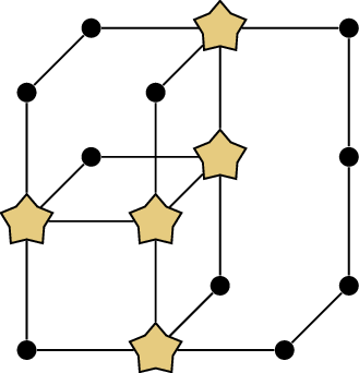
\(K_5\) is not
planarAn unsatisfying extensionA subdivision of \(K_5\)
Non-planar graphs based on \(K_5\)
But we can consider stranger things than just subgraphs. Take a look
at the graph in Figure 22.2(c),
for example. This graph does not have \(K_5\) as a subgraph: it has \(5\) vertices in all the same places as
Figure 22.2(a), but one of the edges is
missing. In place of that long edge is a path through some entirely new
vertices.
If we could draw it in the plane, we could
simply erase the dots on the long path, and get a drawing of \(K_5\).
We can generalize this construction. We say that to
subdivide an edge \(xy\) in a graph \(G\) means to create a new vertex \(z\) and replace edge \(xy\) by edges \(xz\) and \(yz\). (In a diagram, this corresponds to
drawing a dot representing \(z\) in the
middle of edge \(xy\).)
A subdivision of a graph \(G\) is a graph that can be obtained from
\(G\) by subdividing edges zero or more
times. (We consider \(G\) itself to be
a subdivision of \(G\).)
Motivated by Figure 22.2(c) and our argument for it,
what is the relationship between subdivisions and planarity?
If \(H\)
is a subdivision of \(G\), then \(G\) is planar if and only if \(H\) is planar: subdividing edges does not
change planarity.
There is a reason why we have focused on two specific graphs that are
not planar: the graphs \(K_5\) and
\(K_{3,3}\). That reason is the
following theorem, proved in 1930 by Casimir Kuratowski [67]:
Theorem 22.7 (Kuratowski’s theorem). A graph
\(G\) is planar if and only if it \(G\) does not contain a subdivision of \(K_5\) or \(K_{3,3}\).
Thus, subdivisions of \(K_5\) and
\(K_{3,3}\) are the only reasons why a
graph might fail to be planar. (Strictly speaking, I should write,
“\(G\) does not contain a copy of a subdivision
of \(K_5\) or \(K_{3,3}\)”, but nobody is that strict about
it, so I won’t be, either.)
Kuratowski’s theorem is another example of a theorem that lets us
concisely identify a reason why a problem in graph theory might have no
solution. This is not necessarily related to how hard a problem is; it
might be quite hard to find a plane embedding of a large graph, and it
might also be hard to find a subdivision of \(K_5\) or \(K_{3,3}\) inside it. However, once you have
a plane embedding, you can show it to anyone else, and instantly (or
very quickly) convince them that a graph is planar. Working directly
from the definition, there is not a lot you can show someone to quickly
convince them that a graph is not planar.
That’s exactly what Kuratowski’s theorem provides. The subdivisions
of \(K_5\) and \(K_{3,3}\) are obstacles to planarity. But
Kuratowski’s theorem mostly isn’t about telling us that they’re
obstacles: we already knew that part. If we believe that \(K_5\) and \(K_{3,3}\) are not planar, then we can know
that their subdivisions are not planar just by an argument like the one
we used for Figure 22.2(c).
No, Kuratowski’s theorem is about guarantees: it tells us that these
obstacles are the only ones we need to worry about.
I will not give you a proof of Kuratowski’s theorem. However, I will
show you how we can look for a subdivision of \(K_5\) or \(K_{3,3}\) in a graph that is not too large.
(If the graph is very large, then the task should be delegated to a
computer, but it helps to have some understanding of what the computer
could be trying to do.)
A non-planar exampleA \(K_{3,3}\)
subdivisionA \(K_{5}\)
subdivision
Showing that a graph is not planar using Kuratowski’s
theorem
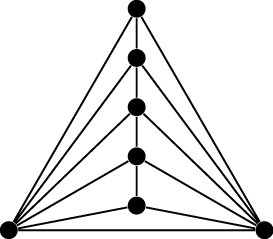
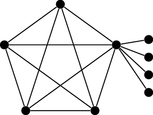
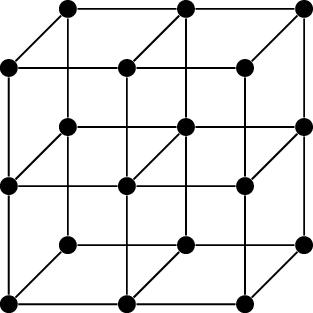
The example I will use is the graph in Figure 22.3(a), which I
will refer to as \(G\) for the rest of
this section. A subdivision of \(K_{3,3}\) inside \(G\) is shown in Figure 22.3(b), and a subdivision of
\(K_5\) in Figure 22.3(c). But how do we find
them?
Must both kinds of subdivisions exist in
\(G\), if it is not planar?
Not necessarily; Kuratowski’s theorem only
promises one of the two kinds of subdivisions. Even if both exist, we
don’t need to find both!
A first step might be to decide whether it is a subdivision of \(K_{3,3}\) or a subdivision of \(K_5\) that we want. If it exists, the
subdivision of \(K_5\) might be easier
to look for, because \(K_5\) has fewer
vertices. However, \(K_5\) has five
vertices of degree \(4\), and this
remains true for every subdivision of \(K_5\). If we’re testing a graph \(G\) with fewer vertices of degree \(4\) or more, we can give up on finding a
subdivision of \(K_5\), and focus on
\(K_{3,3}\). But \(G\) has enough degree-\(4\) vertices (and even two degree-\(5\) vertices) to find both.
In either case, we should begin by deciding which vertices will be
the “key” vertices of the subdivision: the vertices of degree \(3\) or \(4\), as opposed to the vertices of degree
\(2\) in the middle of subdivided
edges. It is a good idea to pick central and high-degree vertices of the
graph, to make it easier to find the paths later. A natural first choice
is one of the two “center” vertices of \(G\). (Call these vertices \(x\) and \(y\), for future reference.)
If we did not know whether \(G\) is
planar, we might also spend some time trying to find a plane embedding
of \(G\). This can also tell us
something, even if we fail! For example, after trying for a while, you
might be able to find a plane embedding of almost all of \(G\), which is missing the edge \(xy\) between the two center vertices.
What would such an embedding tell us?
Since \(G-xy\) is planar, it does not contain a
subdivision of \(K_{3,3}\) or \(K_5\). Therefore whatever subdivision we
hope to find in \(G\) must use edge
\(xy\) somehow.
It is not, logically speaking, necessary for vertices \(x\) and \(y\) to be two of the key vertices of the
subdivision. But it already seemed like a good idea to use these
vertices before, so we might as well start with that theory.
It might take some trial and error to place the remaining key
vertices. It is often a good idea to place as many of them close by as
possible, so that they can be connected directly by edges; then, only a
few long paths are necessary to draw the remaining connections.
It can help to switch between different ways of thinking about the
graphs we’re subdividing—especially \(K_{3,3}\), where we can either imagine the
bipartition with three vertices on each side, or the hexagon with three
chords. For a subdivision of \(K_5\),
we can break down the process of finding it into stages:
Choose \(x\) and \(y\) to be our first two vertices.
Use edge \(xy\) as an edge of
the subdivision, but also find three more longer \(x-y\) paths, sharing no other
vertices.
From each of those \(x-y\)
paths, choose a vertex to be a key vertex of the subdivision. Now, find
a cycle through those three vertices, using no other the vertices used
in previous stages.
A similar breakdown into stages could also work in other
examples.
Graph minors
Another useful operation that preserves the planarity of a graph is
edge contraction. If \(xy\) is an edge
of graph \(G\), the graph \(G \bullet xy\) (also sometimes denoted
\(G/xy\)) is the graph obtained
from \(G\) by deleting vertices \(x\) and \(y\) and adding a new vertex \(z\) adjacent to every vertex which, in
\(G\), was adjacent to either \(x\) or \(y\). The operation of going from \(G\) to \(G
\bullet xy\) is called contracting edge \(xy\).
In some applications, it makes sense to define \(G \bullet xy\) as a multigraph. In that
case, for every edge between a vertex \(w\) and either \(x\) or \(y\) in \(G\), there is an edge between \(w\) and \(z\) in \(G
\bullet xy\); if there are multiple edges between \(x\) and \(y\), and only one of them is contacted, the
remaining edges become loops at \(z\).
In our case, loops and parallel edges are not relevant to track, so we
will keep \(G \bullet xy\) a simple
graph.
Intuitively, given a plane embedding of \(G\), we obtain a plane embedding of \(G \bullet xy\) by first erasing everything
within a small distance of edge \(xy\)
(including the endpoints \(x\) and
\(y\)). Within the erased region, draw
vertex \(z\), and change the trajectory
of every edge formerly incident to \(x\) or \(y\), so that instead it heads to \(z\) once it enters the erased region.
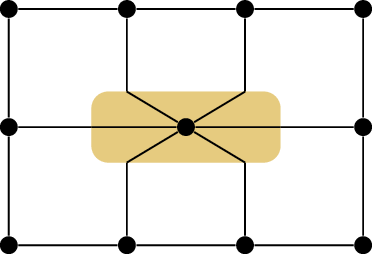
Figure 22.4(a) shows an example of this
intuitive idea, contracting an edge in a \(3\times 4\) grid graph.
Contracting an edgeA \(K_{3,3}\)
minorA \(K_5\)
minor
Examples of edge contractions and minors
Contracting edges is almost, but not quite, the reverse operation of
subdividing edges. If we subdivide an edge \(xy\) (creating a new vertex \(z\)) and then contract edge \(xz\) (calling the combined vertex \(x\)) then we obtain the original graph
again. However, contracting edges can do more than just undo edge
subdivisions, when both endpoints of the contracted edge have degree
\(3\) or more.
We say that a graph \(H\) is a
minor of another graph \(G\)
if it is a subgraph of a graph obtained from \(G\) by contracting edges zero or more
times. If \(G\) is planar, then every
minor of \(G\) is also planar, because
contracting edges will not affect planarity, and neither will going from
\(G\) to a subgraph.
Rather than think of a minor \(H\)
as the result of a sequence of operations done to \(G\), it can help to trace back where every
vertex of \(H\) comes from.
What is the simplest “origin story” of a
vertex of \(H\)?
It could have been a vertex of \(G\) to begin with.
What is next simplest?
A vertex of \(H\) could have started as an edge of \(G\).
What else could have happened?
A vertex of \(H\) could be the result of contracting an
edge whose endpoints were themselves the results of edge contraction(s).
We could have an arbitrarily large set of vertices in \(G\) that all collapse down to one vertex in
\(H\).
There is only one restriction on the set of vertices that collapse
down to one vertex in \(H\). Such a set
only shrinks due to contracting an edge between two of its vertices, so
if we can get it down to a single vertex, it’s because the set was
originally a connected subgraph of \(G\). So, we can identify the vertices of
\(H\) with disjoint connected subgraphs
of \(G\); if two vertices of \(H\) are adjacent, then the corresponding
subgraphs of \(G\) must have at least
one edge between them.
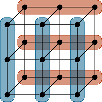
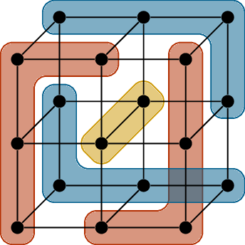
Figure 22.4(b) and Figure 22.4(c) show two examples of this.
Well, to be precise, they show only the subgraphs which are to be
contracted to vertices. In Figure 22.4(b),
the three vertical (blue) subgraphs become one side of \(K_{3,3}\), and the three horizontal (red)
subgraphs become the other side. To verify that we really do get a \(K_{3,3}\) minor, we need to check that
between each red vertex and each blue vertex, there is at least one
edge. Verifying a \(K_5\) minor takes
less explanation: in Figure 22.4(c),
we need to check that there is an edge between every pair of the \(5\) circled regions.
Why is finding a \(K_{3,3}\) minor or a \(K_5\) minor in a graph \(G\) interesting?
It shows that \(G\) is not planar: if \(G\) were planar, then all its minors would
be planar, which is not true of \(K_{3,3}\) or \(K_5\).
Klaus Wagner was the first to study graph minors in 1937 [103]. Among other results, he
proved the analog of Kuratowski’s theorem for graph minors:
Theorem 22.8 (Wagner’s theorem). A graph \(G\) is planar if and only if it does not
have a minor isomorphic to \(K_{3,3}\)
or \(K_5\).
As a characterization of planar graphs, Wagner’s theorem follows from
Kuratowski’s theorem: if \(G\) contains
a subdivision of \(K_{3,3}\) or \(K_5\), then by contracting all the edges
along paths in that subdivision, we can obtain a \(K_{3,3}\) or \(K_5\) minor. As far as we’re concerned in
this book, Wagner’s more significant contribution is the concept of
graph minors. Not all minors arise from subdivisions; in fact, it’s
possible to find a minor isomorphic to \(H\) in a graph which does not contain any
subdivisions of \(H\). So looking for a
\(K_{3,3}\) minor or a \(K_5\) minor is easier than looking for a
subdivision—once you’re comfortable with the definition of a minor.
Outside the study of planar graphs, Wagner’s work proved to be a
greater influence on graph theory, because classifying graphs using
their minors turned out to be a much more useful approach than
classifying graphs using their subdivisions.
Overlap graphs
A different approach to testing whether a graph is planar was first
described in 1959 by Tutte [100]. It is less well-known than Kuratowski’s
theorem, but in my opinion, it is easier to use in small examples, and
it can be the basis for efficient algorithms for planarity testing, as
well. What’s more, it is not just a way to prove that a graph is not
planar; it can help find a plane embedding.
The idea is similar to the approach we took in the previous chapter
to prove that \(K_{3,3}\) is not
planar. It begins by choosing a cycle in the graph we want to test for
planarity. A Hamilton cycle works best, but of course Hamilton cycles
can be hard to find, and we don’t want to turn an easier problem into a
harder problem! We can try the test with any cycle; however, the longer
it is, the better.
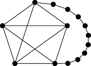
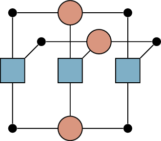
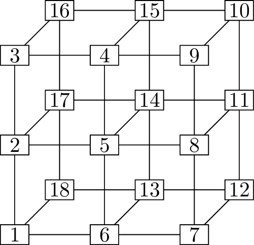
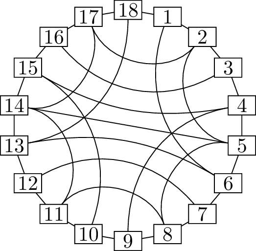
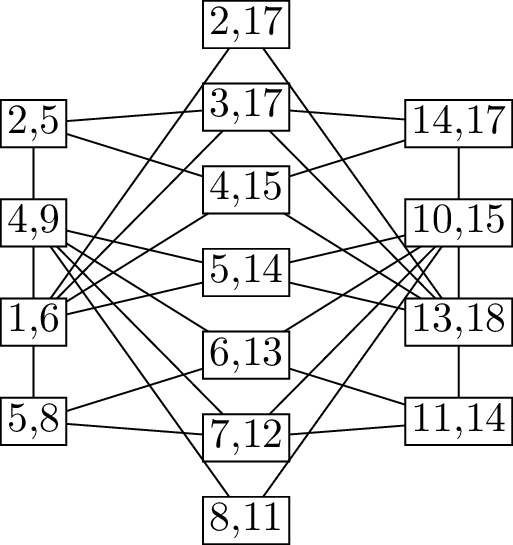
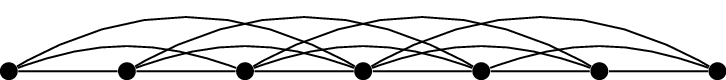
A vertex labelingA Hamilton cycleIts overlap graph
Showing that a graph is not planar using overlap
graphs
As an example, I will show you how this approach works on the graph
\(G\) in Figure 22.3. I have drawn it again
with the vertices labeled in Figure 22.5(a)
for two reasons: for ease of use, and also to point out a Hamilton
cycle. In Figure 22.5(b), that Hamilton cycle is
drawn around a circle, and this picture is good to keep in mind for
intuition.
In a hypothetical plane embedding of \(G\), this cycle (and any other cycle) must
appear as a closed loop of some sort. The rest of \(G\) must be drawn somewhere either inside
that closed loop or outside it. In this example, “the rest of \(G\)” is just the edges which are not part
of the cycle.
In general, given the graph \(G\)
and a cycle \(C\), let \(S\) be the set of vertices on \(C\). We gather the vertices and edges of
\(G\) which are not on \(C\) into fragments, defined as
follows:
Every edge of \(G\) whose
endpoints are both in \(S\) is a
fragment.
Each connected component of \(G-S\), together with the edges it has to
\(S\), is a fragment.
The motivation behind this definition is that a fragment is something
that must either be drawn entirely inside \(C\) in a plane embedding of \(G\), or else entirely outside it: it cannot
cross \(C\). For two different
fragments, on the other hand, we can make different decisions. In our
example, all fragments are edges, because \(C\) is a Hamilton cycle.
Why shouldn’t we have defined edges like
\(\{2,5\}\) and \(\{2,17\}\), which share an endpoint, to be
part of the one fragment?
Because we don’t have to draw them on the
same side of the cycle: to draw edge \(\{2,5\}\) inside the cycle and edge \(\{2,17\}\) outside it, no edges need to
cross.
The decisions that we make for different fragments are not entirely
independent. For example, edge \(\{1,6\}\) and edge \(\{2,17\}\) would intersect if we drew them
both inside the Hamilton cycle, or both outside. To keep track of this
information, we define a new graph, called the overlap graph of
the cycle \(C\). Its vertices are
fragments, and they are adjacent if they “overlap”: if they cannot be
drawn on the same side of \(C\).
A practical definition of the overlap graph in our case is that it
has a vertex for each edge not part of \(C\); two vertices are adjacent if, in
Figure 22.5(b), they cross. This remains a
perfectly good visual rule in general, but we’d like a combinatorial
rule, because a computer cannot look at a drawing and see if two edges
cross. The combinatorial rule for when two fragments overlap is
this:
There are four vertices \(w, x, y,
z\) appearing in that cyclic order around the cycle \(C\).
One fragment includes an edge to vertex \(w\) and an edge to vertex \(y\); this may be satisfied by the fragment
being edge \(wy\).
The other fragment includes an edge to vertex \(x\) and an edge to vertex \(z\); this may be satisfied by the fragment
being edge \(xz\).
The overlap graph in our example is shown in Figure 22.5(c).
Guided by the overlap graph, we must choose for each fragment whether
to draw it inside \(C\) or outside
\(C\). The rule is that if two fragment
are adjacent in the overlap graph, then one of them must be inside \(C\), and the other must be outside \(C\).
In terms of the overlap graph, what are we
trying to find?
A \(2\)-coloring, or bipartition! The fragments
we decide to draw inside \(C\) are one
side of the bipartition, and the fragments we decide to draw outside
\(C\) are the other side.
We know from Chapter 13 that we can efficiently
test if the overlap graph is bipartite, and Theorem 13.1 tells us that the
overlap graph is either bipartite, or contains a cycle of odd length.
That cycle is our proof that the graph cannot be drawn in the plane!
Is there a cycle of odd length in the
overlap graph in Figure 22.5(c)?
Yes: for example, the fragments \(\{1,6\}\), \(\{4,9\}\), and \(\{5,14\}\) form such a cycle.
If the overlap graph were bipartite, would
that be enough to conclude that \(G\)
is planar?
Not in general: it’s also possible that a
single complicated fragment cannot be drawn together with \(C\) without crossing, regardless of what
other fragments are doing. The overlap graph will not detect this.
However, in an example like this one, where \(C\) is a Hamilton cycle, deciding which
fragments are inside and which fragments are outside \(C\) is all that there is to finding a plane
embedding. A bipartition of the overlap graph tells us exactly how to
draw \(G\).
If the overlap graph is not bipartite, then it can also guide us to
finding a subdivision of \(K_5\) or
\(K_{3,3}\). The very simplest case is
what we found in this example: three edges \(\{1,6\}\), \(\{4,9\}\), and \(\{5,14\}\) which all overlap. In that case,
the cycle \(C\) together with those
three edges is a subdivision of \(K_{3,3}\).
In more complicated cases, more work needs to be done, but the
overlap graph can still simplify the search. Take the cycle \(C\), and the fragments forming an odd cycle
in the overlap graph: just this portion of the graph alone is not
planar, so it is all that is necessary to find a subdivision of \(K_5\) or \(K_{3,3}\).
Practice problems
The two graphs below were used as an example in the previous
chapter.
One of these is planar, and the other one is not.
Identify the planar graph, and draw a plane embedding.
Using one of the tools in this chapter, prove that the other
graph is not planar.
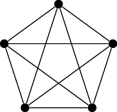
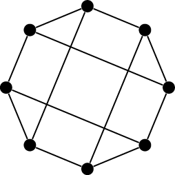
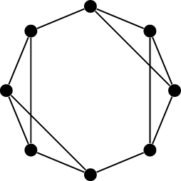
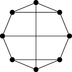
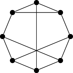
The five connected \(3\)-regular
graphs with \(8\) vertices are all
shown below. Determine which of them are planar, and which are not.
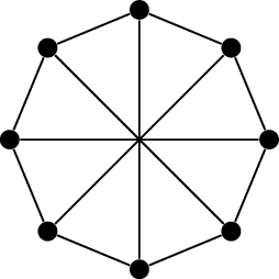
Prove that the Petersen graph is not planar in four different
ways:
By finding a subdivision isomorphic to \(K_{3,3}\).
By finding a minor isomorphic to \(K_5\).
By finding a long cycle in the Petersen graph for which the
overlap graph is not bipartite.
What is the maximum number of edges in an \(n\)-vertex planar graph if we know it has a
plane embedding with two faces of length \(6\)?
Let \(G\) be a connected graph
with \(n\) vertices and \(n+2\) edges. Prove that \(G\) is planar.
Let \(G\) be a graph with \(n\) vertices and \(n+3\) edges obtained by starting with the
cycle graph \(C_n\) and adding \(3\) more edges.
When is \(G\) planar, and when is
\(G\) not planar?
The graph in Figure 22.3(a) is a \(1 \times 2 \times 2\) three-dimensional
grid graph. In general, the \(a \times b
\times c\) grid graph has vertices which are \(3\)-dimensional points \((x_1, x_2, x_3)\) with \(x_1 \in \{1,2,\dots,a\}\), \(x_2 \in \{1,2,\dots,b\}\), and \(x_3 \in \{1,2,\dots,c\}\); two vertices are
adjacent if they are at distance \(1\)
from each other. Thinking of Figure 22.3(a) as a \(3\)-dimensional drawing can give you an
idea of what an \(a\times b\times c\)
grid graph looks like.
For which \(a\), \(b\), and \(c\) is the \(a\times b\times c\) grid graph
planar?
(Putnam 2007) Let a triangulated polygon be a plane embedding in
which every face except the outer face must have length \(3\). Prove that there is a function \(f(n)\) such that if the outer face of a
triangulated polygon has length \(n\),
and every vertex not on the boundary of the outer face has degree at
least \(6\), then the triangulated
polygon has at most \(f(n)\)
faces.