This chapter begins with many examples of analyzing concrete graphs
to find Hamilton cycles, or prove that none exist. The second half of
this chapter is more theoretical. If you are reading this book on your
own, you should feel free to skip to the section on tough graphs as soon
as you feel like you’ve had enough of the discussions that come before
it. If you are teaching from this book, then you can give more of the
concrete examples for a gentle introduction, or leave your students to
read them on your own if your goal is to set a faster pace.
The problem of identifying Hamiltonian graphs is the first of the
“hard problems” we will consider in this book. What do I mean by this?
Well, most precisely put, it is an issue of complexity theory: all the
“hard problems” covered in this part of the textbook are so-called NP-complete problems. You may have heard of
the “P versus NP problem”, an open problem in computer
science whose solution is worth $1 000 000. Finding an efficient
algorithm to solve an NP-complete
problem, or proving that such an algorithm does not exist, would earn
you that million-dollar prize!
This is not a textbook on complexity theory, however, so I will not
go into the details. For us, the consequence of tackling hard problems
is that we will not be able to solve them efficiently, or prove theorems
with simple if-and-only-if conditions describing when they have a
solution. Instead, we will prove partial guarantees, lower and upper
bounds, and discuss algorithms that only sometimes work.
Knight’s tours
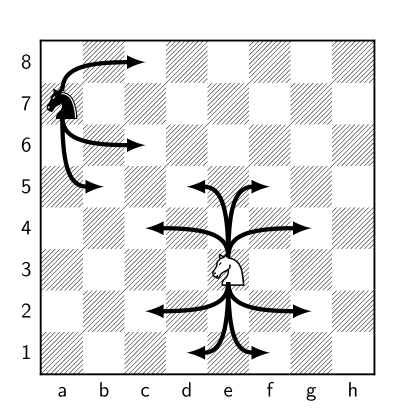
A knight is a chess piece that moves either by taking one step
vertically and two steps horizontally, or by taking two steps vertically
and one step horizontally, as shown in Figure 17.1(a). A knight in the middle of the
board can move to a total of \(8\)
different squares, though this number is reduced if the knight is near
the edges of the board.
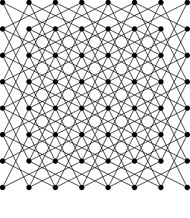
How a knight moves in chessThe graph of knight moves
Chess, knights, and graph theory
For the purpose of graph theory, Figure 17.1(b) is
the correct way to represent how a knight moves in chess. This is the
\(64\)-vertex graph with a vertex for
each square of the chessboard, where two vertices are adjacent if a
knight can move from one square to the other. In this chapter, we will
just call this graph the \(8\times
8\) knight graph.
A knight’s tour is a sequence of knight moves that visits every
square of the chessboard exactly once. Finding a knight’s tour is a
famous mathematical chess puzzle. A slightly harder variant is the
problem of finding a closed knight’s tour: here, after visiting every
square, the knight must make one final move and end at the square where
it started. Both problems have been studied extensively long before
graph theory, both with generic methods and ones specialized to the
chessboard [6]. For
example, in 1832, H. C. von Warnsdorff proposed the short rule, “Start
anywhere, and always move to the space from which the number of moves to
unvisited squares is smallest.” This is quite likely (though not
certain) to produce a knight’s tour; it is also a reasonable heuristic
for the general problem we are about to study.
Graph-theoretically, the knight’s tour problem is the problem of
finding a path or cycle in the \(8\times
8\) knight graph that contains every vertex of the graph. In
general, we say:
Definition 17.1. A Hamilton path
(or spanning path) in a graph is a path that passes through every vertex
of the graph. A Hamilton cycle or (or spanning cycle)
in a graph is a cycle that passes through every vertex of the
graph.
Usually, Hamilton cycles are considered to be the more fundamental
object in graph theory, because they have a symmetry that paths lack:
every vertex plays an identical role. As a result, graphs with Hamilton
cycles are the ones we give a special name.
Definition 17.2. A graph is called
Hamiltonian if it has a Hamilton cycle.
(Actually, there is also a term for graphs that have a Hamilton path:
they are called traceable. This term is much less commonly used.)
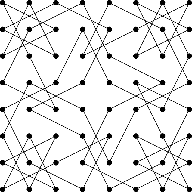
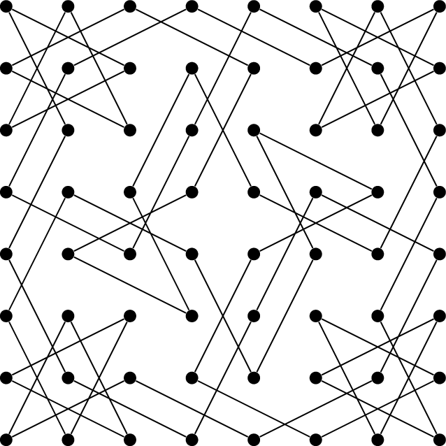
Figure 17.2 shows two interesting
subgraphs in the \(8\times 8\) knight
graph. Both of these were found by Dan Thomasson [96], whose website features an impressive
collection of knight’s tours.
Is this a Hamilton cycle?Is this a Hamilton cycle?
Two symmetric subgraphs of the \(8\times 8\) knight graphHowever, only one of the diagrams in
Figure 17.2 shows a Hamilton cycle.
Which one, and what’s wrong with the other one?
Figure 17.2(b)
shows the Hamilton cycle. In Figure 17.2(a),
every vertex has degree \(2\), but the
edges don’t form a single cycle: there are two connected
components!
Both diagrams in Figure 17.2 do show a \(2\)-factor of the \(8\times 8\) knight graph: a spanning subgraph in which every vertex has degree \(2\). Every Hamilton cycle is a \(2\)-factor, but not vice versa: a Hamilton
cycle must also be connected!
In Chapter 16, we saw the term \(1\)-factor used as a synonym for a
perfect matching: a spanning subgraph in which every vertex has degree
\(1\). Algorithmically, a \(2\)-factor is not much harder to find than
a perfect matching. On the other hand, a Hamilton cycle is much harder
to find. There is no known efficient algorithm, and no characterization
like Tutte’s theorem (Theorem 16.1) of
when a Hamilton cycle exists.
Does the \(8\times 8\) knight graph have a \(1\)-factor, or perfect matching?
Yes; one way to be sure without doing any
additional work is that we can take every other edge in the knight’s
tour shown in Figure 17.2(b),
and get a perfect matching. You might also be able to find some nicely
symmetric perfect matchings from scratch.
Two examples
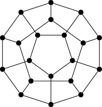
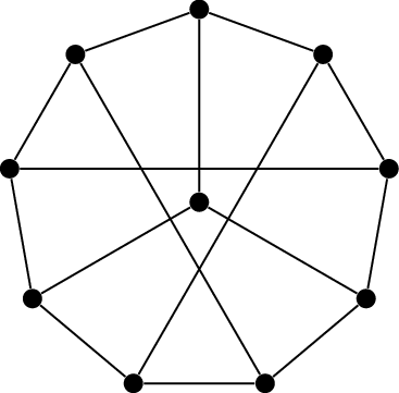
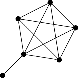
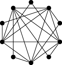
The dodecahedron graphThe Petersen graph
Are these graphs Hamiltonian?
Before we develop any general theory, let’s consider two examples:
the two graphs in Figure 17.3. One
of these graphs is Hamiltonian; the other is not. (Try them for yourself
before you read my explanation, and see what you think.)
The dodecahedron graph in Figure 17.3(a) has a historical
connection to Hamilton cycles. The mathematician William Rowan Hamilton
was a big fan of the dodecahedron; in the 1850s, he invented a puzzle
called the “Icosian Game”, which was effectively to find a Hamilton
cycle in the dodecahedron graph [6]. Although Hamilton’s interest in the puzzle
was more related to his study of abstract algebra, the Icosian Game is
the reason why we refer to spanning cycles as Hamilton cycles.
There is no obvious starting point to the puzzle, so I will give you
an “in” with some mathematical trickery.
As a \(3\)-dimensional shape, the dodecahedron has
\(12\) faces, each of which is a
regular pentagon. A Hamilton cycle in the dodecahedron graph uses
several edges from each pentagon. What is the average number of edges
used per pentagon?
Since the graph has \(20\) vertices, a Hamilton cycle has \(20\) edges. Each edge is also an edge
geometrically: an edge between two faces. So if we add up the number of
edges of the cycle on each pentagon, we will get \(40\): each edge will be counted twice.
There are \(12\) pentagons, so the
average number of edges per pentagon is \(\frac{40}{12} = \frac{10}{3}\).
Is it possible that there is no pentagon
from which we use \(4\) edges?
No. We can’t use all \(5\) edges from a pentagon—then our cycle
would end early. But we also can’t use only \(3\) or fewer edges from all pentagons: then
every pentagon would be below average, which is impossible.
The pentagons are all alike. (Formally, as in Chapter 2, we should say that
there is an automorphism of the dodecahedron graph that can turn any
dodecahedron into any other.) So we can arbitrarily decide that the
“front” pentagon will be the one in which \(4\) edges are used. This leads us to the
partial cycle in Figure 17.4(a).
Step 1Step 2Step 3
Solving the “Icosian Game”
From here, we can make two other deductions.
Our partial cycle is really a path with
two ends. How should we continue from those ends?
We can’t use the edge connecting them,
because then our cycle would end early. So we have to take the only
remaining edges: the ones going outward.
Which edges incident to the topmost vertex
should be part of the cycle?
There is no choice here: the vertex below
the topmost vertex already has degree \(2\), so it can’t accept any more edges. We
must use the two edges going left and right.
Applying the same logic to several other vertices on the perimeter,
we arrive at a bigger partial solution: the one shown in Figure 17.4(b).
At this point, one more “symmetry breaking” step is necessary. From
the bottom vertex in the diagram, we must use either the edge going left
or the edge going right. Which one? Well, it can’t possibly matter: both
the diagram, and our partial solution so far, have left-right symmetry!
So we can arbitrarily pick the edge going right to get one possible
solution; its mirror image will contain the edge going left,
instead.
After this choice, there are several more forced decisions like ones
we already made: once we use two edges out of a vertex \(x\), if \(xy\) is the third edge, then it cannot be
part of the Hamilton cycle, which forces our hand at vertex \(y\). Repeating these steps is all that’s
necessary to arrive at Figure 17.4(c),
the complete solution.
As you see from this example, finding a Hamilton cycle really is more
like solving a puzzle than solving a math problem. Although deductions
like these can often handle small graphs with enough low-degree
vertices, they are not reliable. We might have to make guesses and
backtrack if we fail, which is a slow and tedious process.
Rather than attempt such a backtracking solution for the Petersen
graph, I will show you a different style of argument.
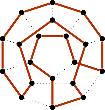
Proposition 17.1. The Petersen graph is not
Hamiltonian.
Proof. This proof will rely on just two properties of the
Petersen graph. First, it is \(3\)-regular, which can be checked quickly
by looking at Figure 17.3(b). Second, as we checked
in Lemma 5.3, it
contains no cycles of length \(3\) or
\(4\).
Now, we proceed in an unusual way. Rather than starting with the
Petersen graph and looking for a Hamilton cycle, let’s start with the
cycle and look for the Petersen graph!
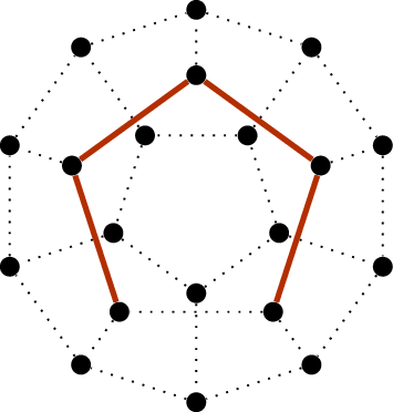
What do I mean? Well, if there were any Hamilton cycle in the
Petersen graph, then we would be able to arrange the vertices around a
regular decagon whose edges are the edges of that cycle. This would look
like the diagram in Figure 17.5(a)—with five more edges we
haven’t placed yet completing the diagram of the \(15\)-edge Petersen graph. For example, from
the topmost vertex, exactly one of the three dashed edges must exist, we
just don’t know which one. (We need a third edge from that vertex to
give it degree \(3\), but any edge
other than the three dashed edges would create a short cycle.)
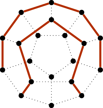
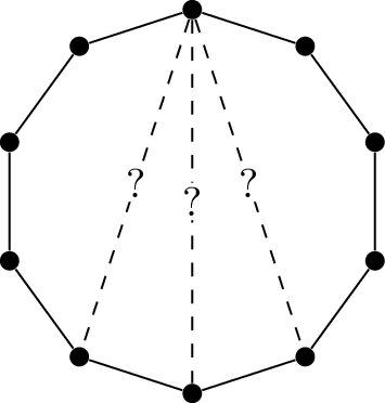
Suppose we pick the left dashed edge. Then we arrive at Figure 17.5(b), and we can ask the same
question for the bottom-most vertex…
Which of the three dashed edges in
Figure 17.5(b) can we use, if we want to
eventually complete the picture to a diagram of the Petersen graph?
None of them! They all create a \(3\)-cycle or \(4\)-cycle.
So we cannot pick the left dashed edge (or, by the same argument, the
right one). We must pick the edge going directly across. Since there’s
nothing special about the top vertex, the same argument applies to every
vertex: the only way we can hope to obtain the Petersen graph is by
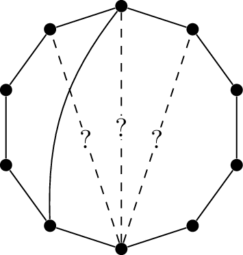
joining each vertex to the vertex directly opposite. This gives us the
graph in Figure 17.5(c).
Why is the graph in Figure 17.5(c) not the Petersen
graph?
It, too, has cycles of length \(4\): starting from any vertex, take a step
across, a step clockwise, another step across, and a step
counterclockwise.
Since all possible attempts to expand a \(10\)-vertex cycle to get a Petersen graph
fail, we conclude that the Petersen graph has no \(10\)-vertex cycle as a subgraph: it is not
Hamiltonian. ◻
Tough graphs
The proof of Proposition 17.1
is rather long. I can’t honestly tell you that the Petersen graph is an
unusually bad example; for many graphs, finding a Hamilton cycle or
proving that one does not exist is even harder. However, there are also
many graphs for which we can give a quick argument to rule out a
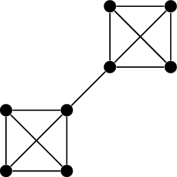
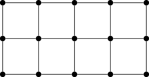
Hamilton cycle. Four of them are shown in Figure 17.6.
Four graphs which are not HamiltonianWhy is the lollipop graph in Figure 17.6(a) not Hamiltonian?
It has a leaf: a Hamilton cycle could not
possibly enter that vertex and leave it.
Why is the barbell graph in Figure 17.6(b) not Hamiltonian?
The edge joining the two copies of \(K_4\) is a bridge; by Lemma 9.2, it is not part of any
cycles. But without using it, a cycle can’t contain vertices from both
copies of \(K_4\).
Why is the book graph in Figure 17.6(c) not Hamiltonian?
Between visits to every “page” of the book
(the vertices of degree \(2\)), a cycle
must pass through at least one vertex of the “spine” (the vertices of
degree \(5\)). But there are only \(2\) vertices in the spine, so a cycle
cannot visit all \(4\) pages.
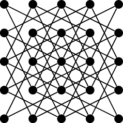
Why is the \(5\times 5\) knight graph in Figure 17.6(d) not Hamiltonian?
Remember the black-and-white covering of a
chessboard? On a \(5\times 5\)
chessboard, there would be \(13\)
squares of one color, and \(12\) on the
other. A knight always moves to squares of a different color (put
differently, the knight graph is bipartite), so a cycle will visit an
equal number of squares of each color: it can’t visit all \(25\) vertices.
Surprisingly, all four arguments are special cases of one result!
We say that a graph \(G\) is
tough if, for any \(k\ge 1\),
deleting \(k\) vertices from \(G\) results in at most \(k\) connected components. You might think,
from this definition, that proving that a graph is tough is a headache
involving lots of casework: there are too many ways to delete some
number of vertices from a graph! In general, you’d be right.
In some cases, it’s not so bad. Here is a lemma that proves that the
cycle graph \(C_n\) is tough without
any casework at all—and, as a bonus, it comes with a mini-review of
Chapter 10.
Lemma 17.2. For all \(n
\ge 3\), the cycle graph \(C_n\)
is tough.
Proof. The cycle graph \(C_n\) has only one cycle: the entire graph.
So as soon as we delete any vertices from it, we get a graph with no
cycles, which we know as a forest. Specifically, if we delete \(k\) vertices from \(C_n\), we get an \((n-k)\)-vertex forest. Each deleted vertex
has degree \(2\) in \(C_n\), so it costs us at most two edges.
Therefore the forest we are left with has at least \(n-2k\) edges.
Why do I say “at most” and “at least”;
shouldn’t every vertex we delete cost us both edges incident to that
vertex?
We might delete both endpoints of an edge,
in which case we shouldn’t count the edge as removed twice.
By a result from much earlier in this book, Proposition 10.3, the number of
connected components in a forest is the number of vertices minus the
number of edges. In this case, this is at most \((n-k) - (n-2k) = k\). Therefore deleting
\(k\) vertices results in a graph with
at most \(k\) components, proving the
lemma. ◻
Starting at \(C_n\) is useful,
because it gives us a connection to Hamiltonian graphs. This is a result
of Václav Chvátal, who defined tough graphs in 1973 for this very
purpose [16].
Corollary 17.3. All Hamiltonian graphs are
tough.
Proof. Every \(n\)-vertex
Hamiltonian graph \(G\) contains a copy
of \(C_n\) as a subgraph: that’s what a
Hamilton cycle is! We can think of \(G\) as this Hamilton cycle, together with
some extra edges it didn’t use.
By Lemma 17.2, if we delete \(k\) vertices from the Hamilton cycle, the
result will have at most \(k\)
connected components. What happens if we delete those same vertices from
\(G\)? Those same connected components
will still be connected, but it’s possible that the extra edges will
join some of them together into larger components. This can only reduce
the number of connected components, so there are still at most \(k\); therefore \(G\) is tough. ◻
The most profitable way to use Corollary 17.3 is
in the form of its contrapositive: if a graph is not tough, then it is
not Hamiltonian. If a graph is not tough, then there is a short proof of
that fact: simply say which \(k\)
vertices must be deleted to leave \(k+1\) or more connected components. (It is
a short proof, not an easy proof, because finding those \(k\) vertices may be hard.)
For example, none of the graphs in Figure 17.6 are
tough—and the sets of vertices we must delete to prove this are closely
related to our earlier arguments proving that none of these graphs are
Hamiltonian. This unifies our previous arguments into a single idea.
Corollary 17.3 is a necessary condition: to
be Hamiltonian, a graph must be tough. However, it is not sufficient, so
we cannot always rely on it. The Petersen graph—a thorn in the side of
every graph theorist—is a counterexample.
Proposition 17.4. The Petersen graph is
tough.
Proof. As we saw in Chapter 5,
the Petersen graph has many automorphisms, and in particular, it has an
automorphism taking any vertex to any other vertex. Due to this
symmetry, it’s enough to see what happens when the vertices we delete
from the Petersen graph include the vertex at the center of Figure 17.3(b), which we will call
\(x\).
If we delete \(x\) alone, the
remaining graph is connected, so the definition of a tough graph holds
so far. What’s more, we can see from the diagram in Figure 17.3(b) that the remaining graph
is Hamiltonian: we get a Hamilton cycle by going around the perimeter of
the diagram. By Corollary 17.3,
this graph is tough. So if we delete \(x\) and \(k\) more vertices from the Petersen graph,
we’re left with at most \(k\) connected
components. Since we’ve deleted \(k+1\)
vertices, that’s even slightly stronger than what we need to conclude
that the Petersen graph is tough. ◻
Sufficient conditions
It is also possible to find conditions for a graph to be Hamiltonian
that are sufficient, but not necessary. That is, if a graph \(G\) satisfies these conditions, we can be
sure that it has a Hamilton cycle; however, if \(G\) does not satisfy these conditions, we
learn nothing.
What’s the point, then? Well, we can look for conditions that are
easy to check. When faced with a concrete problem, we can begin by
checking a few such conditions, and if we’re lucky, this will tell us
that \(G\) is Hamiltonian right away.
Otherwise, we may have no choice but to embark on a tedious journey full
of backtracking.
A promising place to start looking for such conditions is the degree
sequence of \(G\). Computing the degree
of every vertex may take some time, if the graph is large, but it is not
a computationally challenging problem: we can even do it by hand, just
by looking at a diagram. At the same time, the degrees of the vertices
of \(G\) tell us a lot about the
structure of \(G\), so we can hope to
learn something about Hamilton cycles in \(G\), as well.
Historically, the first such result was a 1952 theorem by Gabriel
Dirac [23] (the son of
Paul Dirac, the quantum physicist). More results followed, and
eventually, the essence of the proof was distilled into a rather
peculiar statement, proven by John Bondy and Václav Chvátal in
1976 [8].
Theorem 17.5. In a graph \(G\) with \(n\) vertices, let \(s\) and \(t\) be two non-adjacent vertices with \(\deg_G(s) + \deg_G(t) \ge n\). If \(G+st\) is Hamiltonian, then so is \(G\).
Is it possible that \(G\) is Hamiltonian, but \(G+st\) is not?
No: adding an edge can never destroy a
Hamilton cycle. We could have stated Theorem 17.5 as an if-and-only-if
condition: \(G+st\) is Hamiltonian if
and only if \(G\) is Hamiltonian.
What is going on here? Well, there are many works of fiction in which
the hero is granted special powers by a magic item. Later in the story,
the magic item is lost, and the hero is distressed—only to discover that
the item wasn’t necessary to have the special powers. The magic was
really inside the hero the whole time! The statement of Theorem 17.5 is similar: the graph \(G\) is granted the special power of being
Hamiltonian by the magic edge \(st\).
However (provided that edge \(st\)
satisfies the degree condition) the graph \(G\) didn’t need that edge: the Hamilton
cycle was really inside \(G\) the whole
time.
Theorem 17.5 tries to help us by giving us
a different problem to solve: instead of checking whether \(G\) is Hamiltonian, we can check whether
\(G+st\) is Hamiltonian.
How can this possibly help us?
Well, \(G+st\) has one more edge, so finding a
Hamilton cycle in \(G+st\) might be
easier. A single edge might not make a difference, but if we apply
Theorem 17.5 repeatedly, we can hope to
turn a graph with a well-hidden Hamilton cycle into a graph with many
blindingly obvious Hamilton cycles.
Let’s prove the theorem first, though.
Proof of Theorem 17.5. Take a Hamilton cycle
in \(G+st\). If edge \(st\) is not part of that cycle, we’re done:
it also exists in \(G\). If edge \(st\) is part of that cycle, then deleting
that edge leaves an \(s-t\) Hamilton
path in \(G\). Let this path be
represented by the walk \((x_1, x_2, \dots,
x_n)\) where \(x_1 = s\) and
\(x_n = t\).
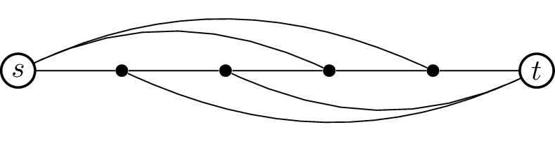
Our goal is to find an alternate way to complete the path \(P\) to a Hamilton cycle in \(G\), without using edge \(st\). All we really know about \(G\) is that, because \(\deg_G(s) + \deg_G(t) \ge n\), there must
be many other edges incident to \(s\)
or \(t\). (There might be other edges,
too, but we cannot count on them.) In short, the subgraph of \(G\) we have available to work with might
look something like the diagram in Figure 17.7(a).
\(P\) together with all
edges incident to \(s\) or \(t\)
Edges in the set \(L\)Edges in the set \(R\)
The cycle in \(G\)
Turning the \(s-t\) path in
the proof of Theorem 17.5
into a cycle
For every edge incident to either \(s\) or \(t\), something special happens: we obtain a
different Hamilton path, which uses that edge, but leaves out one edge
of \(P\). Here are the two ways this
can happen:
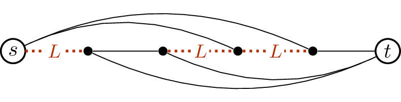
If \(sx_i \in E(G)\) for some
\(i\), then add edge \(sx_i\) to \(P\) and delete edge \(x_{i-1}x_i\). The resulting graph is an
\(x_{i-1} - t\) Hamilton path.
We define the set \(L\) (for “left”)
to be the set of all edges of \(P\)
that can be left out in this way: \(L =
\{x_{i-1} x_i : sx_i \in E(G)\}\). These are highlighted in
Figure 17.7(b).
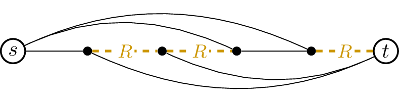
If \(x_{i-1} t \in E(G)\) for
some \(i\), then add edge \(x_{i-1}t\) to \(P\) and delete edge \(x_{i-1}x_i\). The resulting graph is an
\(s - x_i\) Hamilton path.
We define the set \(R\) (for
“right”) to be the set of all edges of \(P\) that can be left out in this way: \(R = \{x_{i-1} x_i : x_{i-1} t \in E(G)\}\).
These are highlighted in Figure 17.7(c).
Can we say anything about the sizes of the
sets \(L\) and \(R\)?
We have \(|L| =
\deg_G(s)\) and \(|R| =
\deg_G(t)\), because for every edge incident to \(s\), we get an element of \(L\), and for every edge incident to \(t\), we get an element of \(R\).
By themselves, edges in \(L\) or in
\(R\) are not anything special, since
we aren’t looking for more Hamilton paths. The magic happens if we find
\(x_{i-1}x_i\) in both sets!
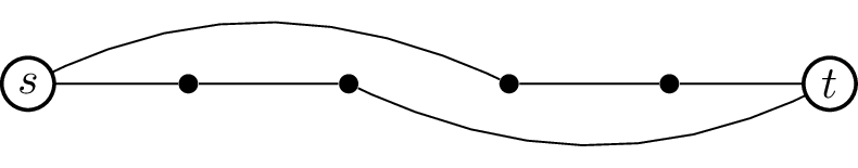
Suppose \(x_{i-1}x_i \in L \cap R\),
so that edges \(sx_i\) and \(x_{i-1} t\) are both present. Let \(C\) be the graph obtained from \(P\) by deleting edge \(x_{i-1}x_i\) and adding both \(sx_i\) and \(x_{i-1}t\), as shown in Figure 17.7(d). This graph \(C\) is a spanning subgraph of \(G\). It is connected: deleting edge \(x_{i-1} x_i\) separated \(P\) into two connected components, but both
\(sx_i\) and \(x_{i-1}t\) join two vertices in different
components, reconnecting the graph. It is \(2\)-regular: compared to \(P\), the degrees of \(s\) and \(t\) go up by \(1\), while all other degrees remain the
same. Therefore \(C\) is a Hamilton
cycle!
The situation is a bit unusual if \(x_1 x_2 \in L \cap R\). What happens?
This would imply that \(x_1x_n = st\) is an edge of \(G\). In principle, this makes a cycle in an
even simpler way: without deleting anything, we just add edge \(st\) to \(P\). However, Theorem 17.5 assumes that this case does
not occur: \(s\) and \(t\) are not adjacent.
Finding an edge in \(L \cap R\) is
why the degree condition on \(s\) and
\(t\) is needed. Since \(|L| = \deg_G(s)\) and \(|R| = \deg_G(t)\), we know that \(|L| + |R| \ge n\) from the hypotheses of
Theorem 17.5. However, \(L\) and \(R\) are both subsets of \(E(P)\), and an \(n\)-vertex path has only \(n-1\) edges, so \(|L \cup R| \le n-1\). Since \(|L \cup R| < |L| + |R|\), there must be
some overlap between \(L\) and \(R\); as we’ve already seen, a single edge
in \(L \cap R\) proves that \(G\) is Hamiltonian, which proves the
theorem. ◻
As an example of applying Theorem 17.5, we
will use it to derive Dirac’s 1952 theorem on Hamilton cycles, with a
sufficient condition based on the minimum degree \(\delta(G)\).
Corollary 17.6. If \(G\) has \(n\ge
3\) vertices and \(\delta(G) \ge
\frac12 n\), then \(G\) is
Hamiltonian.
Proof. The minimum degree condition on \(G\) guarantees that for every two vertices
\(s\) and \(t\) which are not adjacent, we have \[\deg_G(s) + \deg_G(t) \ge \frac12n + \frac12n =
n,\] so the hypotheses of Theorem 17.5
hold. Therefore we can add any edges we like to \(G\) without changing the problem: if we get
a Hamiltonian graph, then \(G\) must
have been Hamiltonian all along.
The edges we will choose to add to \(G\) are all the edges missing from \(G\) (one at a time). Once we’re done, we
get a graph isomorphic to the complete graph \(K_n\). But \(K_n\) is definitely a Hamiltonian graph:
you can visit the vertices in any permutation you like, then go back to
the start, and this will be a Hamilton cycle. Therefore the graph we
started with, \(G\), must also have
been Hamiltonian. ◻
How good is Corollary 17.6? Well, we can compare it to
Proposition 4.3,
which gives \(\delta(G) \ge
\frac{n-1}{2}\) as a sufficient condition for \(G\) to be connected. As we saw in
Chapter 4, that condition is the best
possible: if the minimum degree of \(G\) were any lower than \(\frac{n-1}{2}\), then it would not
necessarily be connected.
When \(\delta(G) = \frac{n-1}{2}\)
exactly, we are in the narrow gap between these two results, where the
graph is guaranteed to be connected by Proposition 4.3,
but not yet guaranteed to be Hamiltonian by Corollary 17.6.
Are there any \(n\)-vertex graphs \(G\) with \(\delta(G) = \frac{n-1}{2}\) which are not
Hamiltonian?
Yes: one example is the slightly
unbalanced complete bipartite graph \(K_{(n-1)/2, (n+1)/2}\). This graph is not
Hamiltonian for the same reason that the \(5\times 5\) knight graph in Figure 17.6(d) was not Hamiltonian.
This tells us that the minimum degree condition of Corollary 17.6 is also the best possible: we cannot
reduce it any further and still have a true statement.
Practice problems
For each of the graphs below, find a Hamilton cycle, or explain
why a Hamilton cycle cannot exist.
Show that for all \(n\ge 5\),
the graph \(\overline{C_n}\) (the
complement of the \(n\)-vertex cycle
graph) is Hamiltonian.
Find a \(5\)-vertex graph \(G\) such that neither \(G\) nor \(\overline{G}\) is Hamiltonian.
Find a Hamilton cycle in the cube graph \(Q_3\).
Prove that the hypercube graph \(Q_n\) has a Hamilton cycle for all \(n \ge 3\), by induction on \(n\).
A Gray code is an alternate binary encoding of numbers with a
useful property: to go from the encoding of \(k\) to the encoding of \(k+1\), only one bit needs to be
changed.
Explain how to obtain a Gray code for the numbers \(0, 1, \dots, 2^n-1\) using a Hamilton cycle
in \(Q_n\).
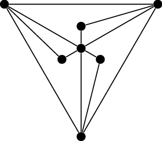
In Chvátal’s original paper defining tough graphs [16], the following example
is given:
Prove that this graph is not Hamiltonian.
Prove that this graph is tough.
Let \(G\) be a bipartite graph
with bipartition \((A,B)\). Prove that
if there is a subset \(S \subseteq A\)
with \(|N(S)| < |S|\), then \(G\) cannot be Hamiltonian. (This statement
is also a consequence of the statement of the next problem, but it can
be proved directly.)
Prove that every tough graph with an even number of vertices (not
necessarily bipartite) has a perfect matching.
Let \(G\) be an arbitrary graph,
and let \(H\) be the graph obtained by
adding a new vertex to \(G\), adjacent
to all vertices which already existed in \(G\). Prove that \(G\) is traceable (\(G\) has a Hamilton path) if and only if
\(H\) is Hamiltonian (\(H\) has a Hamilton cycle).
(This argument is the reason why we do not spend much time thinking
about traceable graphs and Hamilton paths: we can use it to take almost
any fact about Hamilton cycles and turn it into a fact about Hamilton
paths, instead.)
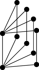
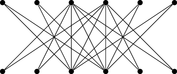
A complete tripartite graph is formed by taking three groups of
vertices \(A\), \(B\), and \(C\), then adding an edge between every pair
of vertices in different groups: this is a generalization of complete
graphs and complete bipartite graphs. We write \(K_{a,b,c}\) for the complete tripartite
graph with \(|A|=a\), \(|B|=b\), and \(|C|=c\). For example, below are diagrams of
\(K_{2,4,5}\) (left) and \(K_{2,3,6}\) (right).
One of these graphs is Hamiltonian. Find a Hamilton cycle in that
graph.
The other graph is not Hamiltonian. Give a reason why it does not
have a Hamilton cycle.
Generalize: find and prove a rule that tells you when \(K_{a,b,c}\) is Hamiltonian. You may assume
\(a \le b \le c\).
Prove that all graphs with the degree sequence \(7, 7, 7, 7, 7, 7, 5, 5, 2\) are
Hamiltonian.
Find a general condition on degree sequences \(d_1, d_2, \dots, d_n\) which guarantees
that all graphs with that degree sequence are Hamiltonian, and which
generalizes your argument from part (a).
(BMO 2011) Consider the numbers \(1, 2,
\dots , n\). Find, in terms of \(n\), the largest integer \(t\) such that these numbers can be arranged
in a row so that all consecutive terms differ by at least \(t\).