In the previous three chapters, we discussed matchings in bipartite
graphs; here, we are going to take another chapter to consider matchings
in general graphs. This division is not because the generalization is
easy, but because it is hard. We will have to do quite a bit of work
just to prove Tutte’s theorem (Theorem 16.1): the
equivalent of Hall’s theorem in cases where the graph is not necessarily
bipartite.
There is a lot more that we’re going to leave undone. We proved
Kőnig’s theorem which deals with the size of a maximum matching; we will
not prove the Tutte–Berge formula, which generalizes Tutte’s theorem to
a Kőnig-type result. We used an algorithm to find maximum matchings in
bipartite graphs. There is a more general algorithm, known as the
blossom algorithm, which can handle non-bipartite graphs, but we will
not discuss it; it is considerably more complicated. If you would like
to learn more about matchings, I recommend Lovász and Plummer’s book
Matching Theory[70].
Compared to the material on Tutte’s theorem, the second half of the
chapter on \(1\)-factorizations is less
intense, and gives some graph-theoretical solutions to problems that
come up in real life. A more relaxed path through this chapter is to
learn about Tutte sets and the statement of Tutte’s theorem, then dive
into \(1\)-factorizations and the
geometric proof of Theorem 16.3.
There are a lot of other problems about factorizations I could have
included instead of the section on increasing walks. In the end, though,
I felt that many people could write a chapter about decomposing \(K_n\) into triangles or Hamilton cycles,
but if I did not mention this beautiful problem in my textbook, it is
not likely that someone else would write about it in theirs.
Tutte sets
In the case of bipartite graphs, we have a complete list of all the
reasons that a perfect matching might fail to exist: the violations of
Hall’s condition. We can summarize these violations as problems of
insufficiency: some vertices do not have enough neighbors for us to get
a perfect matching.
If our graphs don’t have to be bipartite, a second reason that we
might not have a perfect matching appears, and that is parity. The
complete graph \(K_{99}\), or indeed
\(K_{2n+1}\) for any \(n\), does not have a perfect matching, even
though it has all the edges we could wish for, simply because the number
of vertices is odd. Each edge in a matching covers \(2\) vertices, and so the number of vertices
covered by a matching is always even.
Why didn’t we need to worry about parity
when proving theorems about bipartite graphs?
In a graph with bipartition \((A,B)\), we already know that a perfect
matching only exists if \(|A|=|B|\).
When this happens, the total number of vertices is guaranteed to be
even.
If we only had to worry about whether the total number of vertices is
odd or even, that wouldn’t be so bad. But there are examples showing
that our life can be even worse:
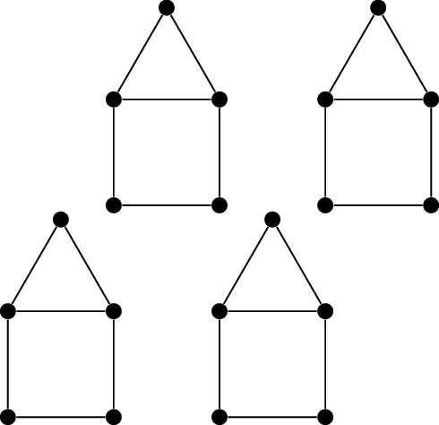
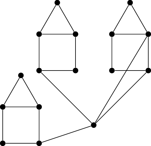
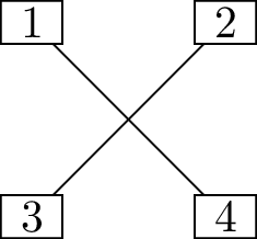
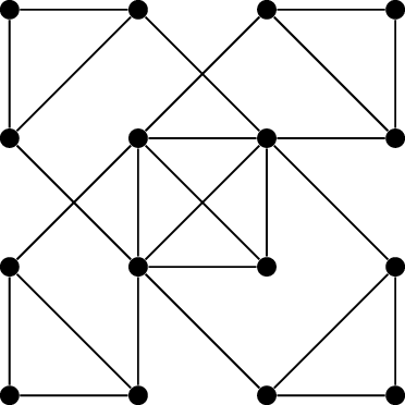
Four housesThree houses and one more vertex
Obstacles to the existence of a perfect
matchingIn Figure 16.1(a), the
total number of vertices is even, and yet there’s still a parity issue
stopping us from having a perfect matching. How?
Each house is a connected component with
an odd number of vertices, so it has no perfect matching, and different
houses cannot help each other.
We will use this idea throughout this chapter, and so we will say
that a connected component with an odd number of vertices is an odd
component, for short. However, odd components all by themselves are
not the only problem.
In Figure 16.1(b),
there is a parity issue even though the graph has no odd components.
How?
Each of the three houses has no perfect
matching on its own, and the extra vertex can be matched to only one of
the houses.
We can imagine that the three houses in Figure 16.1(b) are on fire, and the vertex in
place of the fourth house is a superhero that can put the fires out.
However, the superhero can only be in one place, and cannot put out all
the fires. This problem is a combination of parity and insufficiency: we
have three parity problems in the graph, but only one vertex that can
help us fix them.
We can think of Hall’s theorem (Theorem 15.1) as
saying that if a bipartite graph does not have a perfect matching, then
we can summarize why, by giving an example where Hall’s condition fails.
Similarly, we would like to have somewhere to point the finger of blame
when a general graph does not have a perfect matching.
In both examples in Figure 16.1,
we were able to tell a story about what went wrong, but can we
generalize? The generalization was first found in 1947 by William Thomas
Tutte [99].
We say that a set of vertices \(U\)
in a graph \(G\) is a Tutte
set if the graph \(G-U\) has more
than \(|U|\) odd components.
Yes, and the simplest is the empty set!
(This is allowed, and sometimes it is the only option.)
Tutte not only described what we now call Tutte sets, but proved the
following theorem showing that they are the only kind of obstacle to be
found.
Theorem 16.1 (Tutte’s theorem). Every graph \(G\) has a perfect matching if and only if
it has no Tutte set.
As with Hall’s theorem, one direction of Tutte’s theorem is much
shorter than the other, and the proof of that direction is what
motivated our definitions: we defined a Tutte set specifically because
we had an argument in mind for why a graph with a Tutte set could not
have a perfect matching.
Proof of the “only if” direction of Theorem 16.1.
Suppose that \(U\) is a Tutte set in a
graph \(G\), so that \(G-U\) has \(k
> |U|\) odd components. Let \(M\) be a maximum matching in \(G\), and let \(M'\) be the largest subgraph of \(M\) that is also a matching in \(G-U\). Then \(M'\) must leave at least \(k\) vertices of \(G-U\) uncovered: at least one from each odd
component. However, \(M\) cannot do
much better! An edge of \(M\) is
missing from \(M'\) only if it has
an endpoint in \(U\), and there are at
most \(|U|\) such edges; these can
cover at most \(|U|\) of the vertices
of \(G-U\) that \(M'\) left uncovered. Since \(k > |U|\), we know that there are still
some vertices of \(G-U\) that are
uncovered by \(M\); therefore \(M\) is not a perfect matching. ◻
To prove the other direction of Tutte’s theorem, we will not use
Tutte’s original argument, which relied on linear algebra. Instead, we
will see an argument from Lovász and Plummer’s Matching Theory.
We will arrive at it indirectly, by first describing a special class of
graphs called “saturated graphs” for which the proof will be easier.
Saturated graphs
Call a graph \(G\)saturated1 if \(G\) has no perfect matching, but if \(e\) is any edge not already present in
\(G\), then adding \(e\) to \(G\) would create a perfect matching. (This
includes the case of odd complete graphs \(K_{2n+1}\): they are saturated because they
do not have a perfect matching, and there is no edge \(e\) that can be added.)
Starting from any graph that does not have a perfect matching, we can
arrive at a saturated graph by adding edges, one at a time, for as long
as this is possible without creating a perfect matching.
We could add edges to each house to make
it a copy of \(K_5\), and then add
edges from the extra vertex to every vertex of each house.
Figure 16.2 shows several more
examples of saturated graphs. The idea of Tutte sets helps us come up
with more: if we have a Tutte set, we can add any edges that don’t
change its structure.
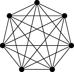
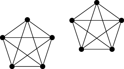
\(K_7\)Two copies of \(K_5\)A nonempty Tutte set
Several examples of saturated graphsIf we start with the four houses in
Figure 16.1(a), and turn each house into a
copy of \(K_5\), is the result
saturated?
No: if we add an edge between two houses,
that increases the size of the matching, but it’s still not a perfect
matching. We can go all the way up to a graph with a copy of \(K_5\) and a copy of \(K_{15}\) before it’s saturated.
Using Tutte’s theorem, we can describe what saturated graphs look
like without too much trouble. (Proposition 16.2 does not describe
saturated graphs completely, but it will be enough for us.)
Proposition 16.2. If a graph \(G\) is saturated, then for some set of
vertices \(U\), \(G\) contains every edge with at least one
endpoint in \(U\), and every edge
between two vertices in the same connected component of \(G-U\).
Proof of Proposition 16.2
using Tutte’s theorem. If a graph \(G\) is saturated, then it has no perfect
matching, so by Tutte’s theorem, it must have a Tutte set \(U\). If an edge \(e\) can be added to \(G\) that would not change \(U\)’s status as a Tutte set, then the
resulting graph \(G+e\) still wouldn’t
have a perfect matching (again, by Tutte’s theorem), which would violate
the definition of a saturated graph. Therefore every such edge must
already exist in \(G\). Which edges are
these?
Well, every edge with at least one endpoint in \(U\) is such an edge, because adding it
wouldn’t affect \(G-U\), so \(U\) would still be a Tutte set. Also, every
edge within a connected component of \(G-U\) is such an edge, because adding it
wouldn’t affect the number of vertices in that component of \(G-U\).
Therefore all such edges are already present in \(G\), proving the proposition. ◻
I made a point to say that this proof used Tutte’s theorem, because
it means that the proof is not good enough for our purposes. What are
those purposes? We are going to reverse the logic, using Proposition 16.2 to prove Tutte’s
theorem!
Proof of Tutte’s theorem
Let’s begin with a fresh proof of Proposition 16.2, so that we can use this
proposition in a proof of Tutte’s theorem without making the argument
circular.
Proof of Proposition 16.2
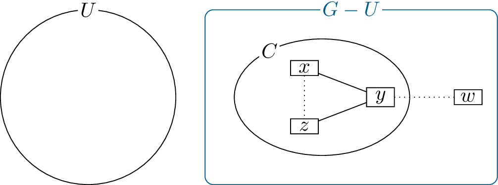
without using Tutte’s theorem. Start by taking \(U\) to be the set of all vertices that are
adjacent to every other vertex.
Suppose that some connected component \(C\) of \(G-U\) does not contain every edge it
possibly could. Choose \(x \in V(C)\)
such that not every vertex of \(C\) is
adjacent to \(x\); let \(z\) be a vertex in \(C\) at distance \(2\) from \(x\), and let \(y\) be their common neighbor. Because \(x,y,z \notin U\), vertex \(y\) must not be adjacent to every vertex;
there must be a fourth vertex \(w\)
(potentially outside \(C\)) not
adjacent to \(y\). This is illustrated
in Figure 16.3.
Vertices \(x,y,z,w\) in the
proof of Proposition 16.2; edges \(xz\) and \(yw\) are not present
We have two ways to make \(G\)
bigger: we could add edge \(xz\), or we
could add edge \(wy\). Because \(G\) is saturated, each of these bigger
graphs must have a perfect matching; because \(G\) has no perfect matching, those two
matchings must each use the added edge. So if we remove the added edge,
we see that \(G\) has two matchings
that are nearly perfect: a matching \(M_{xz}\) that covers all vertices except
\(x\) and \(z\), and a matching \(M_{wy}\) that covers all vertices except
\(w\) and \(y\).
In Chapter 14, to compare two matchings \(M\) and \(N\), we looked at their symmetric
difference \(M\oplus N\). We will do
the same here. We know in general that \(M_{xz} \oplus M_{wy}\) consists of cycles
and alternating paths: paths that alternate between edges of
\(M_{xz}\) and edges of \(M_{wy}\). In this case, we can say even
more.
Where can the alternating paths in \(M_{xz} \oplus M_{wy}\) start and end?
Only at the vertices \(x\), \(y\), \(z\), and \(w\). All other vertices have degree \(1\) in both \(M_{xz}\) and \(M_{wy}\), so they have degree \(2\) or \(0\) in \(M_{xz}
\oplus M_{wy}\).
So \(M_{xz} \oplus M_{wy}\) contains
an \(M_{wy}\)-alternating path that
starts at vertex \(w\) and ends at one
of the three vertices \(x\), \(y\), or \(z\). All three options are good for us:
If it ends at \(y\), then it’s
an \(M_{wy}\)-augmenting path, since it
starts and ends at an uncovered vertex.
If it ends at \(x\) or \(z\), then we can follow up with edge \(xy\) or \(zy\) to go to \(y\); again, we get an \(M_{wy}\)-augmenting path.
If we follow up a \(w-x\) alternating path by going from \(x\) to \(y\), why is that path still
alternating?
We must have arrived to \(x\) by an edge of \(M_{wy}\), because \(M_{xz}\) leaves \(x\) uncovered. Meanwhile, \(xy\) is not an edge of \(M_{wy}\), because \(M_{wy}\) leaves \(y\) uncovered.
By Lemma 14.3, we can use the \(M_{wy}\)-augmenting path to improve \(M_{wy}\) to a perfect matching in \(G\). But we assumed \(G\) was saturated, and didn’t have a
perfect matching! This is the contradiction that finishes the
proof. ◻
Let me explain the reasons behind what’s happened so far. It’s common
that when proving a theorem about graphs that don’t have a property
(such as a perfect matching), it is enough to prove the theorem about
graphs that don’t have the property, but have as many edges as possible:
in our case, about saturated graphs. We’re about to see in a moment that
this is true here: proving Tutte’s theorem will be much easier for
saturated graphs than for graphs with no special properties.
So we want to learn about saturated graphs. Since we suspect that
Tutte’s theorem is true even before we have a proof, we started by using
it to understand what saturated graphs ought to look like. Then, we went
back and proved the same result in legitimate ways, so that it’s no
longer circular reasoning to use it to prove Tutte’s theorem.
Now let’s see if our efforts have paid off!
Proof of the “if” direction of Theorem 16.1. Let
\(G\) be a graph that does not have a
perfect matching.
How can we finish the proof if \(G\) has an odd number of vertices?
In this case, \(U = \varnothing\) is a Tutte set in \(G\), so Tutte’s theorem holds.
So we assume that \(G\) has an even
number of vertices. Then the reason that \(G\) doesn’t have a perfect matching is
simply because it’s missing some edges.
Greedily add edges to \(G\), one by
one, for as long as this does not create a perfect matching, until we
cannot add edges any longer. The result is a saturated graph \(H\) that contains \(G\) as a spanning subgraph.
By Proposition 16.2
applied to \(H\), there is some set of
vertices \(U\) such that \(H\) contains every edge with at least one
endpoint in \(U\), and every edge with
both endpoints in the same connected component of \(H-U\). We will first prove that \(U\) is a Tutte set in \(H\), and then that it is a Tutte set in
\(G\).
Let \(M\) be a maximum matching in
\(H-U\). In every connected component
\(C\) of \(H-U\), all edges are present, so the only
possible reason why \(M\) might not
cover every vertex of \(C\) is
that \(C\) is an odd component. What’s
more, if there are \(|U|\) or fewer odd
components, then we can extend \(M\) to
a perfect matching of \(H\): match
vertices in \(U\) to vertices outside
\(U\) not covered by \(M\), and if any vertices in \(U\) are left, match them to each other. So
there must be more than \(|U|\) odd
components in \(H-U\), which exactly
means that \(U\) is a Tutte set in
\(H\).
Where did we need the assumption that
\(G\) and \(H\) have an even number of vertices?
Otherwise, “if any vertices in \(U\) are left, match them to each other”
might not work: we might end with one vertex uncovered.
Since \(G\) is a subgraph of \(H\), every connected component of \(H-U\) breaks down into one or more
components of \(G-U\). However, an odd
number cannot be the sum of many even numbers; therefore every odd
component of \(H-U\) must contain at
least one odd component of \(G-U\). We
conclude that \(G-U\) has at least
\(|U|\) odd components, which means
that \(U\) is also a Tutte set in \(G\). ◻
1-factorizations
A practical application of matchings in graphs that we have yet to
consider is tournament design. (We will only explore the basics of the
overlap between this field and graph theory.)
Suppose that we would like to organize a round-robin chess
tournament2 between \(n\) players. A single chess game can take a
while, so we want to schedule as many games at the same time as
possible. When \(n\) is even, we can
always begin by dividing \(n\) people
into \(n/2\) arbitrary pairs and
scheduling a game between each pair. This is a perfect matching in \(K_n\), which is not a very difficult
matching problem.
However, this only tells us what to do in the first round; future
rounds are more difficult, because we don’t want to repeat any games. If
the first round is a perfect matching \(M_1\) in \(K_n\), then we would like the second round
to be a perfect matching \(M_2\) in the
complement \(\overline{M_1}\), the
third round to be a perfect matching in \(\overline{M_1 \cup M_2}\), and so on. These
matching problems can easily become impossible if we schedule rounds of
the tournament with no foresight.
For example, with \(6\) players, we
hope to finish in \(5\) rounds, because
each player has \(5\) opponents to
face. However, if our first three matchings are poorly chosen, then they
might leave us with a graph that has no perfect matching of its own. We
would have to ask two people to sit out of the fourth round, and then we
would have to schedule \(6\) rounds
total.
Can this problem really occur? How do we
run a \(6\)-player tournament
badly?
Taking \(V(K_6)\) to be \(\{1,2,3,4,5,6\}\), we might mistakenly
begin with three matchings that all match even numbers to odd numbers:
for example, \(\{12, 34, 56\}\), then
\(\{14, 25, 36\}\), then \(\{16,23,45\}\). Now, the remaining graph
has two odd components and no perfect matching.
Instead of solving this problem one matching at a time, we will have
to solve it all at once: we want to find a decomposition of \(G\), writing at as a union of perfect
matchings that share no vertices. There is a special term for this kind
of decomposition.
Definition 16.1. A \(1\)-factorization of a graph \(G\) is a decomposition of \(G\) into perfect matchings: a
representation \[G = M_1 \cup M_2 \cup \dots
\cup M_k\] where each \(M_i\) is
a perfect matching, and each edge of \(G\) appears in exactly one \(M_i\).
The term “\(1\)-factorization” goes
back to the early days of graph theory, where the idea of a graph was
more algebraic: an edge \(xy\) was
really thought of as the product of two variables \(x\) and \(y\), and a graph was just the product of
such edges. For example, a cycle with vertices \(\{x, y, z\}\) would be the expression \((xy)(xz)(yz)\). Some other modern terms
have their origin in those days. For example, if you simplify the
product that we use to represent our cycle, you get \(x^2 y^2 z^2\); the degree of each variable
(in the algebraic sense) is exactly the degree of the corresponding
vertex (in the graph-theoretic sense)!
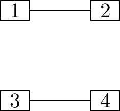
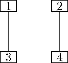
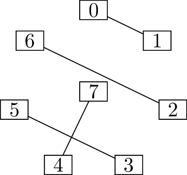
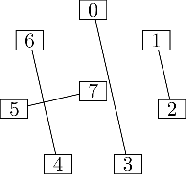
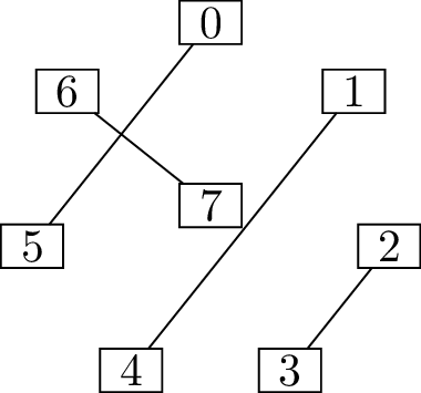
The \(1\)-factor \((x_1x_2)(x_3x_4)\)The \(1\)-factor \((x_1x_3)(x_2x_4)\)The \(1\)-factor \((x_1x_4)(x_2x_3)\)
A \(1\)-factorization of
\(K_4\): three disjoint \(1\)-factors whose product is \(x_1^3 x_2^3 x_3^3 x_4^3\)
Viewed from this point of view, a \(1\)-factorization really is a factorization
of the graph: a way to write it as a product of factors in which every
variable has degree \(1\). (For this
reason, perfect matchings are also sometimes called \(1\)-factors.) For example, the graph \(K_4\), viewed as the product \((x_1x_2)(x_1x_3)(x_1x_4)(x_2x_3)(x_2x_4)(x_3x_4)\),
has the \(1\)-factorization \[\underbrace{(x_1x_2)(x_3x_4)}_{\text{1-factor}}
\cdot
\underbrace{(x_1x_3)(x_2x_4)}_{\text{1-factor}}
\cdot
\underbrace{(x_1x_4)(x_2x_3)}_{\text{1-factor}}.\]Figure 16.4 shows this factorization
in a more modern way.
Of course, what’s important is finding the \(1\)-factorization, not representing it.
Theorem 16.3. The complete graph \(K_n\) has a \(1\)-factorization whenever \(n\) is even.
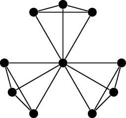
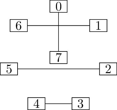
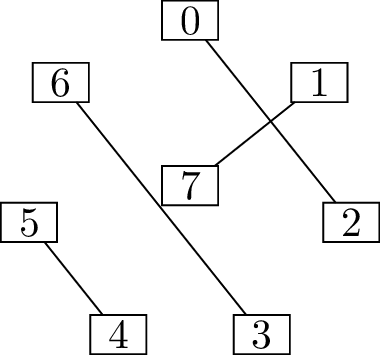
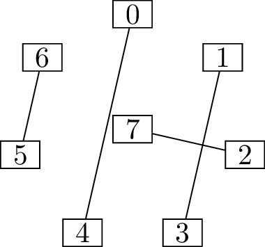
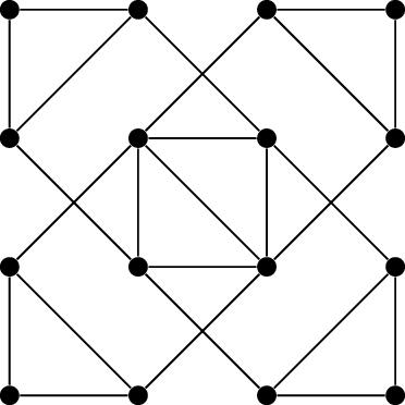
Proof. It is much easier to draw a diagram of the \(1\)-factorization than it is to give a
diagram-free proof. Begin with a diagram of \(K_n\) that places \(n-1\) of the vertices at evenly spaced
points around a circle, and the last vertex in the middle of the circle.
For the \(i^{\text{th}}\) matching
\(M_i\), take the edge between the
middle vertex to the \(i^{\text{th}}\)
vertex around the circle, as well as all edges perpendicular to this
edge in the diagram.
(Figure 16.5 shows an example of this
construction in the case \(n=8\).)
In a way, the diagram also leads to a geometric proof. Name the \(n-1\) matchings after the \(n-1\) radial edges. For each edge \(xy\) between two outer vertices, construct
the diameter perpendicular to \(xy\),
and one half of that diameter will be an edge from the middle vertex.
This tells us which matching contains edge \(xy\); in particular, it tells us that \(xy\) is in exactly one matching. To see
that it’s a matching, we first check that \(xy\) does not share a vertex with the
radial edge perpendicular to it (the lines intersect at the midpoint of
edge \(xy\), not at a vertex). In all
other cases, two edges \(xy\) and \(x'y'\) in the same matching are
parallel: they do not share a vertex because, as lines, they do not
intersect.
For a diagram-free proof, we rely on modular arithmetic instead.
Number the vertices \(0\) through \(n-1\). For each \(i=0,1,\dots,n-2\), define the matching
\(M_i\) to contain the edge \(\{i, n-1\}\) as well as all the edges \(\{i-k \bmod n-1, i+k \bmod n-1\}\) for
\(k=1, \dots, n/2 - 1\). Since the
\(n-1\) values \[i - (n/2 - 1), i - (n/2 - 2), \dots, i-1, i, i+1,
\dots, i + (n/2 - 1)\] are distinct modulo \(n-1\), no vertices are repeated, and
therefore \(M_i\) really is a
matching.
Next, we show that no edge is contained in multiple matchings. This
is true for edges incident to \(n-1\),
since each matching is defined to contain a different one of these
edges. Otherwise, take an edge \(xy \in E(M_i)
\cap E(M_j)\). Since \(xy \in
E(M_i)\), we can write it as \[\{x,y\}
= \{i-k \bmod n-1, i+k \bmod n-1\}\] for some \(k\), so \(x+y
\equiv (i-k) + (i+k) = 2i \pmod{n-1}\). Similarly, since \(xy \in E(M_j)\), then \(x+y = 2j \pmod{n-1}\). But \(n\) is even and \(0 \le i,j \le n-2\), so \(2i \equiv 2j \pmod{n-1}\) can only occur if
\(i=j\).
What goes wrong at this step if \(n\) is odd?
Then \(2i \equiv
2j \pmod{n-1}\) really is possible for two values \(i\) and \(j\). For example, if \(n=7\), we’d be working modulo \(6\), and \(2
\cdot 1 \equiv 2 \cdot 4 \pmod 6\).
From the previous paragraph, it also follows that every edge is
contained in some matching. If there are \(n-1\) matchings, and each contains \(n/2\) edges, then together they contain
\(\frac{n(n-1)}{2}\) edges total, and
we’ve shown that there’s no overlap. But there are only \(\frac{n(n-1)}{2}\) edges in \(K_n\), so we’ve included them all. ◻
In my opinion, the geometric proof is the “real” reason that
Theorem 16.3 is true, but I have
included the number-theoretic proof for completeness. It requires some
background in number theory to follow, but in reality, working modulo
\(n-1\) is just a diagram-free way to
put \(n-1\) evenly spaced points around
a circle.
Now we know how to schedule a round-robin tournament between \(n\) people in just \(n-1\) rounds, if \(n\) is even!
What do tournament organizers do if \(n\) is odd?
In each round, one player gets a “bye” and
sits out. This is equivalent to scheduling an \((n+1)\)-player tournament with one player
named “bye” who doesn’t really exist.
Since \(n+1\) is even whenever \(n\) is odd, adding a fictional player named
“bye” reduces the problem to a case where Theorem 16.3 applies. Of course, with
\(n+1\) players, we require \(n\) rounds, even if one of the players is
fictional. This proves the following corollary:
Corollary 16.4. When \(n\) is odd, the complete graph \(K_n\) has a decomposition into \(n\) matchings which are each nearly perfect
(covering \(n-1\) of the \(n\) vertices).
Many other graphs can be shown to have \(1\)-factorizations. Let’s briefly return to
bipartite graphs to prove one more result, originally also due to
Kőnig [62]:
Theorem 16.5. Every regular bipartite graph has a
\(1\)-factorization.
Proof. By Theorem 15.2, every
regular bipartite graph \(G\) has a
perfect matching \(M\). If \(G\) is \(k\)-regular, then \(G-E(M)\) is \((k-1)\)-regular: every vertex of \(G\) is incident to one edge of \(M\), so its degree goes down by \(1\) in \(G-E(M)\).
Repeat this argument, removing perfect matchings from \(G\) until it is \(0\)-regular, and there are no more edges.
(Formally, this proof should be rephrased as an induction on \(k\); can you see how?) The perfect
matchings removed at each step form a \(1\)-factorization of \(G\). ◻
Increasing walks
The problem of finding a \(1\)-factorization of \(K_n\) was historically first studied by
tournament organizers, not graph theorists. However, that does not mean
it is not useful in graph theory. I encountered the following problem as
a graduate student.
Take the complete graph \(K_n\), and
make it into a weighted graph by giving each edge \(e\) a weight \(c(e)\); in this problem, we will insist
that all the weights should be different. A walk \((x_0, x_1, x_2, \dots, x_l)\) is called an
increasing walk if the weights go up along the walk: if \[c(x_0 x_1) < c(x_1 x_2) < \dots <
c(x_{l-1}x_l).\] What is the longest possible increasing walk?
Well, it depends on the labels. We can have very long increasing walks
if the weights cooperate. Suppose that before choosing edge weights, we
pick a walk \((x_0, x_1, x_2, \dots,
x_l)\) that we’d like to be increasing. Provided the walk does
not repeat any edges, we can make it so! Simply set \(c(x_{i-1}x_i) = i\) for \(i=1,2,\dots,l\).
What is the longest walk in \(K_n\) that does not repeat any edges?
If \(n\)
is odd, then all degrees are even, so \(K_n\) has an Euler tour: a walk of length
\(\binom n2\). If \(n\) is even, then we can delete any
matching and be left with an Eulerian graph, with an Euler tour of
length \(\binom n2 - n/2\).
This is a best-case analysis, and the short solution to it shows us
why worst-case analyses are much more interesting. Instead, let’s ask
the question: what is the longest possible length of an increasing walk
that we can guarantee, no matter what the weights of the edges are?
This problem was first studied by Ron Graham and Daniel Kleitman, who
proved in 1973 [39] that
it was possible to find weighted graphs in which the longest increasing
walk is much shorter.
Proposition 16.6. For all even \(n\), there is a weighted complete graph on
\(n\) vertices in which no increasing
walk has length more than \(n-1\).
Proof. Use Theorem 16.3
to decompose \(K_n\) into \(n-1\) perfect matchings \(M_1\) through \(M_{n-1}\). For each \(i\), and each \(e
\in E(M_i)\), set \(c(e) = i\).
Okay, that doesn’t quite work, because the weights all have to be
different, but it will have the same effect if \(c(e)\) is any number in the interval \([i, i+\frac12]\): we will never end up
comparing two edges in a matching anyway.
An increasing walk in this weighted graph cannot use more than one
edge from any matching \(M_i\). After
taking its first edge from that matching, it cannot immediately take a
second edge, because no two edges in \(M_i\) share an endpoint. So the walk must
follow up by going to a different matching: since the walk is
increasing, it must select an edge from \(M_j\), for some \(j>i\). But this edge has a greater
weight than any edge of \(M_i\), so the
increasing walk can never return to \(M_i\) again.
Since there are only \(n-1\)
matchings, the increasing walk cannot use more than \(n-1\) edges. ◻
Graham and Kleitman proved more than this. They generalized
Proposition 16.6 to work for odd
\(n\) as well, excluding the special
case \(n=3\) and \(n=5\). Moreover, they proved that this
upper bound is always achievable! I will present their solution in a
different style, as described by Peter Winkler [108] and attributed to Ehud Friedman.
Proposition 16.7. In every weighted complete
graph on \(n\) vertices, there is an
increasing walk of length at least \(n-1\).
Proof. Imagine that we put \(n\) different people on the \(n\) vertices of the complete graph. Then,
we call out the edges of the graph one by one, in increasing order of
weight. Whenever we call out an edge \(xy\), the two people standing on vertices
\(x\) and \(y\) trade places, walking along edge \(xy\) in opposite directions.
At the end, we will ask each person to describe the walk they took.
All these walks must be increasing, because all edges were announced in
increasing order. Let \(l_1, l_2, \dots,
l_n\) be the lengths of the \(n\) walks.
How can we express the sum \(l_1 + l_2 + \dots + l_n\) in another
way?
The sum counts each edge of the graph
twice, since two people walk each edge, so it is equal to \(2|E(K_n)|\), which is \(n(n-1)\).
If the lengths \(l_1, l_2, \dots,
l_n\) add up to \(n(n-1)\), then
their average is \[\frac{l_1 + l_2 + \dots +
l_n}{n} = \frac{n(n-1)}{n} = n-1,\] and it is impossible for all
\(n\) lengths to be below average.
Therefore at least one walk must have length at least \(n-1\). ◻
Practice problems
In one of the graphs below, find a perfect matching. In the
other, prove that there is no perfect matching, by finding a Tutte
set.
Theorem 15.2 from
the previous chapter implies that every \(3\)-regular bipartite graph has a perfect
matching.
Prove that the word “bipartite” cannot be left out: give an example
of a \(3\)-regular graph which is not
bipartite, and does not have a perfect matching.
(USAMO 1989) The \(20\) members
of a local tennis club have scheduled exactly \(14\) two-person games among themselves,
with each member playing in at least one game. Prove that within this
schedule there must be a set of \(6\)
games with \(12\) distinct
players.
Use Tutte’s theorem to prove Hall’s theorem.
Let \(o(G)\) denote the number
of odd components in a graph \(G\).
Prove that if \(G\) is a graph and
\(U\) is a subset of \(V(G)\), then \[\alpha'(G) \le \frac12\big({|V(G)| - o(G-U) +
|U|}\big).\] (More is true. The Tutte–Berge formula is a
generalization of Tutte’s theorem saying that the two sides of this
inequality are equal for some set \(U\).)
Prove that if \(G\) is a graph
with an even number of vertices and no perfect matching, then it has a
Tutte set \(S\) with \(o(G-S) \ge |S|+2\).
Suppose that \(2n\) people from
two different \(n\)-person teams
participate in a tournament. Describe how to schedule \(n\) rounds of simultaneous games between
players on opposing teams, so that each person plays once against
everyone on the other team.
(In other words, find a \(1\)-factorization of the complete bipartite
graph \(K_{n,n}\). Theorem 16.5 assures us that one
exists, but doesn’t say what it is.)
Let \(G\) be a copy of \(K_8\) with vertices \(\{000, 001, \dots, 111\}\) (just like the
vertices of the cube graph \(Q_3\)).
For each nonempty subset \(S \subseteq
\{1,2,3\}\), let \(M_S\) be the
matching consisting of all edges in \(G\) whose endpoints differ in the positions
numbered by \(S\). For example, \[E(M_{\{1,2\}}) = \Big\{\{000,110\}, \{001,111\},
\{010, 100\}, \{011, 111\}\Big\}.\] Prove that the seven
matchings \(M_{\{1\}}, M_{\{2\}}, M_{\{3\}},
M_{\{1,2\}}, M_{\{1,3\}}, M_{\{2,3\}}, M_{\{1,2,3\}}\) are a
\(1\)-factorization of \(G\).
Prove that this \(1\)-factorization is not isomorphic to the
one found in Theorem 16.3.
That is, prove that it is not possible to replace the labels \(\{000,001,\dots,111\}\) by \(\{0,1,\dots,7\}\) in any way to turn this
\(1\)-factorization into the one shown
in Figure 16.5.
Define an increasing path to be a path such that one of the walks
representing it is an increasing walk.
We can prove a version of Proposition 16.7 for increasing paths by
changing the rules slightly in that proof. Whenever edge \(xy\) is called out, if the person on \(x\) has already visited \(y\), or the person on \(y\) has already visited \(x\), then both people stay put. This
ensures that at the end, each person’s walk represents an increasing
path.
Suppose that each person walks a path of length at most \(L\). Prove that each person is responsible
for “rejecting” at most \(\frac{L(L-1)}{2}\) edges.
At the end, each of the \(\binom
n2\) edges was either walked by two people or rejected by at
least one person. Use this to prove the inequality \(n \cdot \frac L2 + n \cdot \frac{L(L-1)}{2} \ge
\binom n2\).
Prove \(L \ge
\sqrt{n-1}\).
Graham and Kleitman proved a similar result, but unlike the problem
of increasing walks, the exact worst-case answer is still not known in
the case of increasing paths.
A graph \(G\) is called
claw-free if it does not have a copy of the star graph \(S_4\) as an induced subgraph. In other
words, no vertex \(x \in V(G)\) can
have three neighbors \(y_1, y_2, y_3\)
with no edges between them.
Sumner’s theorem [95]
states that every connected claw-free graph with an even number of
vertices has a perfect matching. Prove this using Tutte’s theorem.
(Here is a hint for one possible solution: choose a careful ordering
\(x_1, x_2, \dots, x_k\) of the
vertices in \(S\), then prove by
induction on \(i\) that the number of
connected components of \(G-S\) with a
neighbor in \(\{x_1, x_2, \dots,
x_i\}\) cannot exceed \(i+1\).)
Footnotes
The word “saturated” is commonly used in graph theory
for this type of definition, but it usually needs to be qualified with
some other adjectives to say what kind of problem \(G\) is saturated for. In this book, we will
not need this term outside this chapter, so I will just say “saturated”
for brevity, even though it’s not as precise.↩︎
“Round-robin”, in case you’re unfamiliar with the
terminology, means that every participant plays a game against every
other participant.↩︎